Converting to NeuroML

On inspection of the model, we see that it has two biophysically detailed cell models:

• the GGN (Giant GABAergic Neuron)

• the KC (Kenyon cell)

Converting the Giant GABAergic Neuron

Step 1) Exporting morphology of the GGN

Let’s start with the GGN first. It’s morphology is defined as an SWC file in this file. One can download this file and view the morphology in a tool, like the HBP morphology viewer.

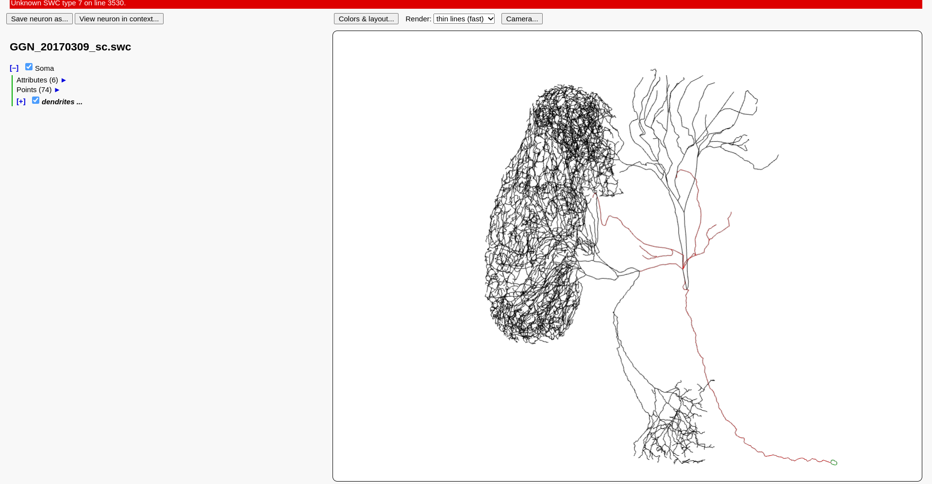
Fig. 66 Visualisation of the GGN in the HBP morphology viewer.

A NEURON HOC script that includes the full morphology and the biophysics is also included.

Let us export the morphology first. pyNeuroML includes the export_to_neuroml2 helper function that exports a cell model in NEURON to NeuroML. We can write a short script to use this function to export the morphology from the provided HOC script.

#!/usr/bin/env python3
"""
Convert cell morphology to NeuroML.

We only export morphologies here. We add the biophysics manually.

File: NeuroML2/scripts/cell2nml.py
"""

import os
import sys

import pyneuroml
from pyneuroml.neuron import export_to_neuroml2
from neuron import h


def main(acell):
    """Main runner method.

    :param acell: name of cell
    :returns: None

    """
    loader_hoc_file = f"{acell}_loader.hoc"
    loader_hoc_file_txt = """
    /*load_file("nrngui.hoc")*/
    load_file("stdrun.hoc")
    xopen("../../NEURON/mb/cell_templates/GGN_20170309_sc.hoc")
    objref cell
    cell = new GGN_20170309_sc()
    """

    with open(loader_hoc_file, 'w') as f:
        print(loader_hoc_file_txt, file=f)

    export_to_neuroml2(loader_hoc_file, f"{acell}.morph.cell.nml",
                       includeBiophysicalProperties=False, validate=False)

    os.remove(loader_hoc_file)
    # Note--a couple of diameters are 0.0, modified to 0.001 to validate the
    # model


if __name__ == "__main__":
    if len(sys.argv) != 2:
        print("This script only accepts one argument.")
        sys.exit(1)
    main(sys.argv[1])

What we’re doing here is using the HOC script to build the cell model in NEURON, and then exporting it to NeuroML. Calling it as python cellmorph2nml.py GGN will create a new file: GGN.morph.cell.nml which contains the morphology of the cell in NeuroML format. Note that while export_to_neuroml2 does allow exporting the biophysics of the cell, it is better to add these manually later once one has gone through and converted the required ion channels and so on.

We can visualise the morphology using the pyNeuroML tools:

pynml-plotmorph -i GGN.morph.cell.nml

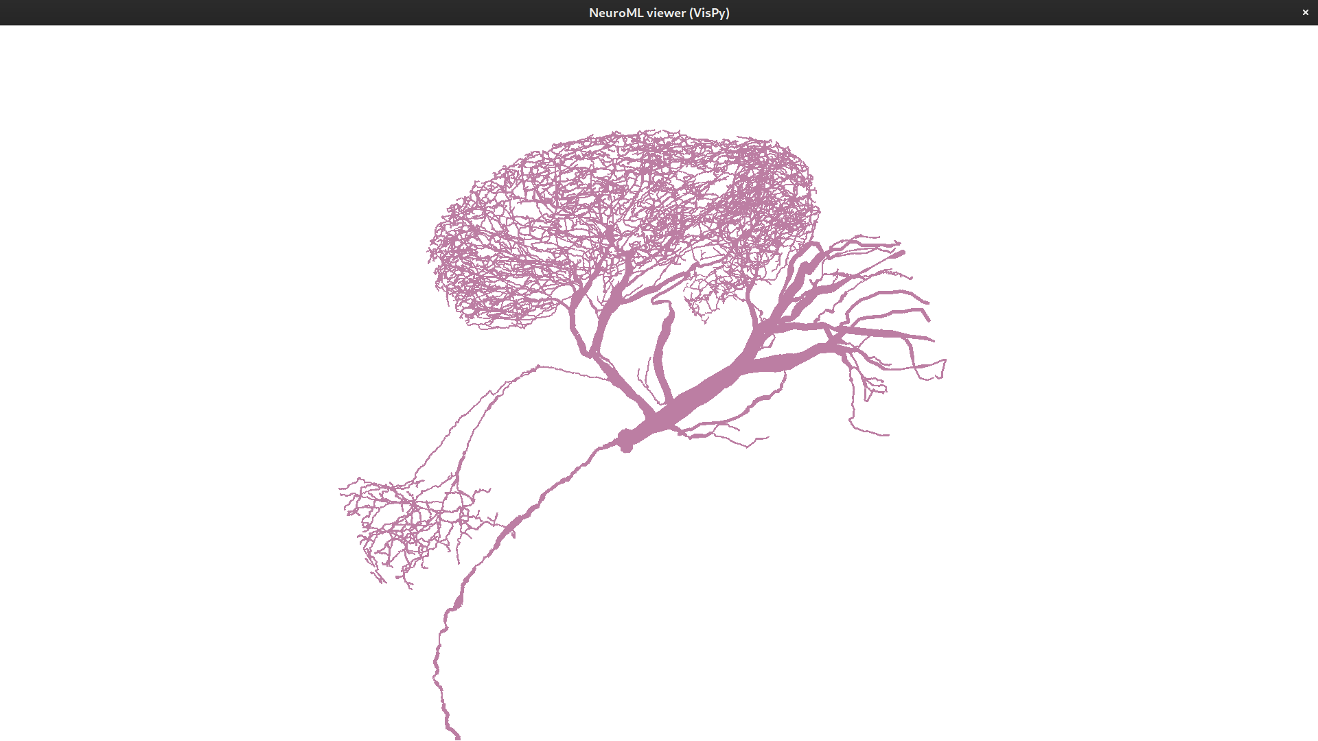
Fig. 67 Visualisation of the GGN using pynml-plotmorph

Step 2) Adding biophysics to the GGN

Now that we have the morphology of the GGN exported, we can add the biophysics. We need to inspect the original model code to learn about the biophysics. In this model, for the GGN cell, the biophysics are included in the HOC script:

proc biophys() {
  forsec all {
    Ra = 100.0
    cm = 1
    insert pas
      g_pas = 0.03e-3   // S/cm2 - as per Laurent et al 1990 RM = 33kohm-cm2
      e_pas = -51
  }
}

As we see here, this is a passive cell without any ion channels. To add the biophysics, we write a simple Python script that will make use of the pyNeuroML API. The complete script is present in the repository:

def load_and_setup_cell(cellname: str):
    """Load a cell, and clean it to prepare it for further modifications.

    These operations are common for all cells.

    :param cellname: name of cell.
        the file containing the cell should then be <cell>.morph.cell.nml
    :returns: document with cell
    :rtype: neuroml.NeuroMLDocument

    """
    celldoc = read_neuroml2_file(
        f"{cellname}.morph.cell.nml"
    )  # type: neuroml.NeuroMLDocument
    cell = celldoc.cells[0]  # type: neuroml.Cell
    celldoc.networks = []
    cell.id = cellname
    cell.notes = cell.notes.replace("GGN_20170309_sc_0_0", cellname)
    cell.notes += ". Reference: Subhasis Ray, Zane N Aldworth, Mark A Stopfer (2020) Feedback inhibition and its control in an insect olfactory circuit eLife 9:e53281."

    [
        default_all_group,
        default_soma_group,
        default_dendrite_group,
        default_axon_group,
    ] = cell.setup_default_segment_groups(
        use_convention=True,
        default_groups=["all", "soma_group", "dendrite_group", "axon_group"],
    )

    # populate default groups
    for sg in cell.morphology.segment_groups:
        if "soma" in sg.id and sg.id != "soma_group":
            default_soma_group.add(neuroml.Include(segment_groups=sg.id))
        if "axon" in sg.id and sg.id != "axon_group":
            default_axon_group.add(neuroml.Include(segment_groups=sg.id))
        if "dend" in sg.id and sg.id != "dendrite_group":
            default_dendrite_group.add(neuroml.Include(segment_groups=sg.id))

    cell.optimise_segment_groups()

    return celldoc


def postprocess_GGN():
    """Post process GGN and add biophysics."""
    cellname = "GGN"
    celldoc = load_and_setup_cell(cellname)
    cell = celldoc.cells[0]  # type: neuroml.Cell

    # biophysics
    # all
    cell.add_channel_density(
        nml_cell_doc=celldoc,
        cd_id="pas",
        ion_channel="pas",
        cond_density="0.00003 S_per_cm2",
        erev="-51 mV",
        group_id="all",
        ion="non_specific",
        ion_chan_def_file="channels/pas.channel.nml",
    )
    cell.set_resistivity("0.1 kohm_cm", group_id="all")
    cell.set_specific_capacitance("1 uF_per_cm2", group_id="all")
    cell.set_init_memb_potential("-80mV")

    # L1 validation
    # cell.validate(recursive=True)
    cell.summary(morph=False, biophys=True)
    # use pynml writer to also run L2 validation
    write_neuroml2_file(celldoc, f"{cellname}.cell.nml")

The load_and_setup_cell function does some basic clean up and set up of the cell. It ensures that the various segments that were exported from NEURON are placed into the conventional segment groups. The postprocess_GGN function then adds the passive biophysics to the cell.

The pas channel is a standard implementation of a passive ion channel. The rest are membrane properties–resistivity, specific capacitance and so on. Once this is set up, we write the cell to a new file.

The GGN cell has now been converted. Since the GGN is a simple passive cell, we won’t test its biophysics just yet.

Converting the Kenyon Cell

The KC cell is defined in the kc_1_comp.hoc file. Whereas the GGN cell had a complex morphology but passive biophysics, the KC cell has very simple morphology—a single compartment—but does contain active channels:

create soma


objref all
proc subsets() { local i
  objref all
  all = new SectionList()
  soma all.append()
}
proc geom() {
     soma {  // Total Cm = 4 pF
        L = 6.366
        diam = 20
    }
}

proc biophys() {
  forsec all {
    Ra = 35.4
    cm = 1
    insert pas
      g_pas = 9.75e-5         // S/cm2
      e_pas = -70             // mV
    insert kv
      gbar_kv = 1.5e-3       // S/cm2
    insert ka
      gbar_ka = 1.4525e-2    // S/cm2
    insert kst
      gbar_kst = 2.0275e-3   // S/cm2
    insert naf
      gbar_naf = 3.5e-2      // S/cm2
    insert nas
      gbar_nas = 3e-3        // S/cm2
      ek = -81.0             // mV
      ena = 58.0               // mV
  }
}

Step 1) Converting ion channels

For this cell, we will first convert the various ion channel models. These are included in the mod folder. An inspection tells us that these are all Hodgkin-Huxley type ion channels that use similar formalisms.

The first thing to do is to generate plots of time courses and steady states of the various ion channels. These can be done easily using pynml-modchananalysis command line tool included in pyNeuroML. We begin with the nas channel:

pynml-modchananalysis -modFile nas_wustenberg.mod nas

This will generate two plots, one for the steady state dynamics (inf), and one for the time course (tau) for activation variables in the channels:

Fig. 68 Time course of activation variables of nas channel, generated with pynml-modchananalysis

Fig. 69 Steady state dynamics of activation variables of nas channel, generated with pynml-modchananalysis

The mod file defining the nas channel is shown below:

Here we have the m and h activation variables. Although they are described in the standard Hodgkin Huxley formalism, in the settables procedure, we can see that their values are only calculated in the range of -120mV to 40mV. The value does not change beyond 40mV. This could be done for a number of reasons. Perhaps the cell’s membrane potential does not go beyond 40mV.

We will attempt to remain faithful to the mod file in our conversion, so we will also incorporate this feature.

Since we know this is a Hodgkin Huxley type channel, we can search the schema to see if there are any elements that can describe it. A search shows us that the ionChannelHH component type exists in the schema/standard. In the schema, this is identical to ionChannel. The usage examples included in the documentation indicate that we can use these elements from the standard to describe the ion channel here. We need to:

• include the m gate, which has 3 sub units (m^3)

• include the h gate, which has 1 sub unit (h^1)

• formalise the equations that are used to calculate the steady state (inf)and time course (tau) for these gates/activation variables.

To begin with, let us ignore the restriction included in the mod file at 40mV. Our NeuroML description will look something like this:

<ionChannel id="nas" type="ionChannelHH" conductance="1pS" species="na">

<!-- some more details to be added here -->

</ionChannelHH>

Now, there are number of different ways of expressing the dynamics of the activation variables. (See this page for an introduction to HH formalism). One can use the values of the forward and reverse rates (called alpha and beta in general) to calculate the steady state and time course. Another possibility is that alpha and beta are not given, and instead the equations for the steady state and time course are. The latter is the case here:

inf = 1 / ( 1 + exp((Vh - V) / s) )

If the rates are given, one can use the gateHHrates component type from the standard. If the steady state and time course are, we can use gateHHtauInf. There are also other components that can be used if a combination of rates and/or steady state and time course are given.

The equation above is in the form of a sigmoid function. Another search in the standard shows us that we have the HHSigmoidVariable component type that can be used to represent a rate that is a sigmoid function. The dynamics tab tells us that the equation is represented as:

x = rate / (1 + exp(0 - (v - midpoint)/scale))

Putting the equation for minf and hinf together with this form:

x = rate / (1 + exp(0 - (v - midpoint)/scale))
minf  = 1.0 / (1 + exp((-30.1 - v) / 6.65))
hinf  = 1.0 / (1 + exp((v + 51.4) / 5.9 ))

We can see that for minf, rate = 1 per ms, scale = 6.65mV and midpoint = -30.1mV. Similarly, for hinf, rate = 1 per ms, scale = -5.9mV and midpoint = -51.4mV.

<ionChannel id="nas" type="ionChannelHH" conductance="1pS" species="na">

    <gate id="m" instances="3" type="gateHHtauInf">
        <steadyState type="HHSigmoidVariable" midpoint="-30.1mV" scale="6.65mV" rate="1" />
        <timeCourse />
    </gate>

    <gate id="h" instances="1" type="gateHHtauInf">
        <steadyState type="HHSigmoidVariable" midpoint="-51.4mV" scale="-5.9mV" rate="1" />
        <timeCourse />
    </gate>
</ionChannel>

The time course is given by:

taum = (taumax - taumin) / (1 + exp((V - Vh1) / s1)) + taumin

Even though this is also a sigmoid, it is not, unfortunately, a standard form. A component type does not exist in the NeuroML standard that can encapsulate this form (It has more parameters, and has an additional + taumin).

This is not a problem, though, because NeuroML can be easily extended using LEMS. We can write a new component type to encapsulate these dynamics based on the LEMS definition of the HHSigmoidVariable component type:

<ComponentType name="HHSigmoidVariable"
               extends="baseHHVariable"
               description="Sigmoidal form for variable equation">
    <Dynamics>
        <DerivedVariable name="x" dimension="none" exposure="x" value="rate / (1 + exp(0 - (v - midpoint)/scale))"/>
    </Dynamics>
</ComponentType>

Our new component will be this, and we will save it in a different file that we can then “include” in the nas channel definition file:

<!-- Saved as RayTau.nml -->
<?xml version="1.0" encoding="ISO-8859-1"?>
<neuroml xmlns="http://www.neuroml.org/schema/neuroml2" xmlns:xsi="http://www.w3.org/2001/XMLSchema-instance" xsi:schemaLocation="http://www.neuroml.org/schema/neuroml2 https://raw.github.com/NeuroML/NeuroML2/development/Schemas/NeuroML2/NeuroML_v2beta4.xsd" id="NeuroML_ionChannel">

    <ComponentType name="Ray_tau"
                  extends="baseVoltageDepTime"
                  description="Tau parameter">

        <Parameter name="max_tau" dimension="time"/>
        <Parameter name="min_tau" dimension="time"/>
        <Parameter name="midpoint" dimension="voltage"/>
        <Parameter name="scale" dimension="voltage"/>
        <Dynamics>
            <DerivedVariable name="t" dimension="time" exposure="t" value="(((max_tau - min_tau) / (1 + exp(0 - (v - midpoint) / scale))) + min_tau)"/>
        </Dynamics>
    </ComponentType>
</neuroml>

Note that it is very similar to the HHSigmoidVariable definition. The only difference is that we have had to define additional parameters to use in our equation. Also note that HHSigmoidVariable extends baseHHVariable which extends baseVoltageDepVariable. However, since we know that tau is a time value, we extend the baseVoltageDepTime component type instead. This is very similar to baseVoltageDepVariable, but is designed for component types producing time values, such as the time course here.

We save this as a different component type (a class), and we will provide it parameters to create our time courses for both m and h activation variables. Our completed file will look like this:

<!-- saved as nas.channel.nml -->
<?xml version="1.0" encoding="ISO-8859-1"?>
<neuroml xmlns="http://www.neuroml.org/schema/neuroml2" xmlns:xsi="http://www.w3.org/2001/XMLSchema-instance" xsi:schemaLocation="http://www.neuroml.org/schema/neuroml2 https://raw.github.com/NeuroML/NeuroML2/development/Schemas/NeuroML2/NeuroML_v2beta4.xsd" id="NeuroML_ionChannel">

    <notes>NeuroML file containing a single ion channel</notes>
    <include href="RayTau.nml" />

    <ionChannel id="nas" type="ionChannelHH" conductance="1pS" species="na">

        <gate id="m" instances="3" type="gateHHtauInf">
            <steadyState type="HHSigmoidVariable" midpoint="-30.1mV" scale="6.65mV" rate="1" />
            <timeCourse type="Ray_tau" min_tau="0.83 ms" max_tau="0.093 ms" midpoint="-20.3 mV" scale="6.45mV"/>
        </gate>

        <gate id="h" instances="1" type="gateHHtauInf">
            <steadyState type="HHSigmoidVariable" midpoint="-51.4mV" scale="-5.9mV" rate="1" />
            <timeCourse type="Ray_tau" min_tau="1.9 ms" max_tau="12.24 ms" midpoint="-32.6 mV" scale="-8.0mV"/>
        </gate>
    </ionChannel>

</neuroml>

Running pynml-channelanalysis nas.nml will generate the graphs for the steady state and time course from our channel definition, and you will see that these are the same as the graphs we generated from the mod files.

We are almost there, but we have a little more work to do here. Remember that the original mod file limited the value of steady state at 40mV? We have not incorporated that into our channel file yet.

Since the HHSigmoidVariable we have used for the steady state does not allow multiple equations, we will write a new component type for the steady state also:

<?xml version="1.0" encoding="ISO-8859-1"?>
<neuroml xmlns="http://www.neuroml.org/schema/neuroml2" xmlns:xsi="http://www.w3.org/2001/XMLSchema-instance" xsi:schemaLocation="http://www.neuroml.org/schema/neuroml2 https://raw.github.com/NeuroML/NeuroML2/development/Schemas/NeuroML2/NeuroML_v2beta4.xsd" id="NeuroML_ionChannel">

    <ComponentType name="Ray_inf"
        extends="baseVoltageDepVariable"
        description="Inf parameter for Ray et al 2020" >

        <Constant name="table_max" dimension="voltage" value="40 mV"/>
        <Parameter name="rate" dimension="none"/>
        <Parameter name="midpoint" dimension="voltage"/>
        <Parameter name="scale" dimension="voltage"/>
        <Dynamics>
            <ConditionalDerivedVariable name="x" dimension="per_time" exposure="x">
                <Case condition="v .gt. table_max" value="(rate / (1 + exp(0 - (table_max - midpoint) / scale)))"/>
                <Case value="(rate / (1 + exp(0 - (v - midpoint) / scale)))"/>
            </ConditionalDerivedVariable>
        </Dynamics>
    </ComponentType>
<neuroml/>

The only difference here is that instead of the DerivedVariable, we have used a ConditionalDerivedVariable that allows conditional dynamics. We have two cases here:

• if v is greater than table_max (which is 40mV), the rate is the value at v=40mV

• otherwise, the rate is calculated from the value of v

1a) Kv, Naf, Kst

The nas channel is now done. If we look at the other channels—naf, kv, and kst—they follow similar formalisms. So, we can re-use our newly created component types, Ray_inf and Ray_tau. In fact, we consolidate them in a single file, RaySigmoid.nml, and “include” this in the channel definition files. For example, here is kv.channel.nml:

<?xml version="1.0" encoding="ISO-8859-1"?>
<neuroml xmlns="http://www.neuroml.org/schema/neuroml2" xmlns:xsi="http://www.w3.org/2001/XMLSchema-instance" xsi:schemaLocation="http://www.neuroml.org/schema/neuroml2 https://raw.github.com/NeuroML/NeuroML2/development/Schemas/NeuroML2/NeuroML_v2beta4.xsd" id="NeuroML_ionChannel">

    <notes>NeuroML file containing a single ion channel</notes>
    <include href="RaySigmoid.nml" />

    <ionChannel id="kv" conductance="1pS" type="ionChannelHH" species="k">

        <notes>
                Implementation of A type K+ channel ( KV ) from Wustenberg DG, Boytcheva M, Grunewald B, Byrne JH, Menzel R, Baxter DA.
                This is a delayed rectifier type K+ channel in Apis mellifera Kenyon cells (cultured).
        </notes>

        <!-- custom component types because the tables in the mod files only go to 40 -->
        <gate id="m" type="gateHHtauInf" instances="4">
            <steadyState type="Ray_inf" rate="1.0" midpoint="-37.6mV" scale="27.24mV"/>
            <timeCourse type="Ray_tau" min_tau="1.85 ms" max_tau="3.53 ms" midpoint="45.0 mV" scale="-13.71mV"/>
        </gate>

    </ionChannel>
</neuroml>

Plots for the steady state and time course are:

Fig. 70 Steady state dynamics of activation variables of kv channel, generated with pynml-channelanalysis

Fig. 71 Time course of activation variables of kv channel, generated with pynml-channelanalysis

In these graphs, the effect of the conditional at 40mV becomes more apparent.

1b) Ka

The last remaining channel is the ka channel. It’s dynamics are defined in the mod file as:

PROCEDURE settables(v (mV)) { 
UNITSOFF
        TABLE minf, hinf, mtau, htau FROM -120 TO 40 WITH 641
        minf  = 1.0 / (1 + exp((-20.1 - v)/16.1))
        hinf  = 1.0 / ( 1 + exp( ( v + 74.7 ) / 7 ) )
        mtau = (1.65 - 0.35) / ((1 + exp(- (v + 70) / 4.0)) * (1 + exp((v + 20) / 12.0))) + 0.35
        htau = (90 - 2.5) / ((1 + exp(- (v + 60) / 25.0)) * (1 + exp((v + 62) / 16.0))) + 2.5
UNITSON
}

The steady state here follows the same formalism, but the time course does not. So, we need to create new component type to encapsulate the time courses here, similar to the Ray_tau component type that we did before:

    <ComponentType name="Ray_ka_tau"
                   extends="baseVoltageDepTime"
                   description="Tau parameter to describe ka">

        <Parameter name="max_tau" dimension="time"/>
        <Parameter name="min_tau" dimension="time"/>
        <Parameter name="midpoint1" dimension="voltage"/>
        <Parameter name="scale1" dimension="voltage"/>
        <Parameter name="midpoint2" dimension="voltage"/>
        <Parameter name="scale2" dimension="voltage"/>
        <Constant name="table_max" dimension="voltage" value="40 mV"/>
        <Dynamics>
            <ConditionalDerivedVariable name="t" dimension="time" exposure="t" >
                <Case condition="v .gt. table_max" value="(max_tau - min_tau) / ((1 + exp(-(table_max + midpoint1) / scale1)) * ( 1 + exp((table_max + midpoint2) / scale2))) + min_tau"/>
                <Case value="(max_tau - min_tau) / ((1 + exp(-(v + midpoint1) / scale1)) * ( 1 + exp((v + midpoint2) / scale2))) + min_tau"/>

            </ConditionalDerivedVariable>
        </Dynamics>
    </ComponentType>

We also add this to our RaySigmoid.nml file. The ka.channel.nml file will, finally, look like this:

<?xml version="1.0" encoding="ISO-8859-1"?>
<neuroml xmlns="http://www.neuroml.org/schema/neuroml2" xmlns:xsi="http://www.w3.org/2001/XMLSchema-instance" xsi:schemaLocation="http://www.neuroml.org/schema/neuroml2 https://raw.github.com/NeuroML/NeuroML2/development/Schemas/NeuroML2/NeuroML_v2beta4.xsd" id="NeuroML_ionChannel">

    <notes>NeuroML file containing a single ion channel</notes>
    <include href="RaySigmoid.nml" />

    <ionChannel id="ka" conductance="1pS" type="ionChannelHH" species="k">

        <notes>
                Implementation of A type K+ channel ( KA ) from Wustenberg DG, Boytcheva M, Grunewald B, Byrne JH, Menzel R, Baxter DA.
                This is transient A type K+ channel in Apis mellifera Kenyon cells (cultured).
        </notes>

        <!-- custom component types because the tables in the mod files only go to 40 -->
        <gate id="m" type="gateHHtauInf" instances="3">
            <timeCourse type="Ray_ka_tau" midpoint1="70mV" midpoint2="2.0mV" scale1="4.0mV" scale2="12.0mV" min_tau="0.35ms" max_tau="1.65ms"/>
            <steadyState type="Ray_inf" rate="1.0" midpoint="-20.1mV" scale="16.1mV"/>
        </gate>

        <gate id="h" type="gateHHtauInf" instances="1">
            <timeCourse type="Ray_ka_tau" midpoint1="60mV" midpoint2="62.0mV" scale1="25.0mV" scale2="16.0mV" min_tau="2.5ms" max_tau="90.0ms"/>
            <steadyState type="Ray_inf" rate="1.0" midpoint="-74.7mV" scale="-7.0mV"/>
        </gate>

    </ionChannel>
</neuroml>

That is all the ion channels converted.

The ion channels are usually the most involved to convert because one must understand their initial descriptions in the mod files. Even though the NMODL language used in mod files does have a well defined structure, like general programming languages, it is free-flowing. This means that different people can write the same dynamics in different ways. On the other hand, NeuroML and LEMS are more formal with more strict structures, and once channels are converted to these formats, they are much easier to understand.

Step 2) Creating the morphology

Since the morphology of the KC is a single compartment, we don’t need to export it from NEURON. We can create it ourselves.

The morphology is given in the HOC script:

proc geom() {
     soma {  // Total Cm = 4 pF
        L = 6.366
        diam = 20
    }
}

We can create this using a Python script:

    celldoc = component_factory(
        "NeuroMLDocument", id="KC_doc"
    )  # type: neuroml.NeuroMLDocument
    cell = celldoc.add("Cell", id="KC", validate=False)  # type: neuroml.Cell
    cell.setup_nml_cell()
    cell.add_segment([0, 0, 0, 20], [0, 0, 6.366, 20], seg_type="soma")

The setup_nml_cell and add_segment methods are part of the Cell class in the standard API.

Now that we have the morphology and the ion channels for the KC, we can add the biophysics to the morphology to complete the cell:

    # biophysics
    # all
    cell.set_resistivity("35.4 ohm_cm", group_id="all")
    cell.set_specific_capacitance("1 uF_per_cm2", group_id="all")
    cell.set_init_memb_potential("-70mV")
    cell.set_spike_thresh("-10mV")

    cell.add_channel_density(
        nml_cell_doc=celldoc,
        cd_id="pas",
        ion_channel="pas",
        cond_density="9.75e-5 S_per_cm2",
        erev="-70 mV",
        group_id="all",
        ion="non_specific",
        ion_chan_def_file="channels/pas.channel.nml",
    )

    # K
    cell.add_channel_density(
        nml_cell_doc=celldoc,
        cd_id="kv",
        ion_channel="kv",
        cond_density="1.5e-3 S_per_cm2",
        erev="-81 mV",
        group_id="all",
        ion="k",
        ion_chan_def_file="channels/kv.channel.nml",
    )
    cell.add_channel_density(
        nml_cell_doc=celldoc,
        cd_id="ka",
        ion_channel="ka",
        cond_density="1.4525e-2 S_per_cm2",
        erev="-81 mV",
        group_id="all",
        ion="k",
        ion_chan_def_file="channels/ka.channel.nml",
    )
    cell.add_channel_density(
        nml_cell_doc=celldoc,
        cd_id="kst",
        ion_channel="kst",
        cond_density="2.0275e-3 S_per_cm2",
        erev="-81 mV",
        group_id="all",
        ion="k",
        ion_chan_def_file="channels/kst.channel.nml",
    )
    # Na
    cell.add_channel_density(
        nml_cell_doc=celldoc,
        cd_id="naf",
        ion_channel="naf",
        cond_density="3.5e-2 S_per_cm2",
        erev="58 mV",
        group_id="all",
        ion="na",
        ion_chan_def_file="channels/naf.channel.nml",
    )
    cell.add_channel_density(
        nml_cell_doc=celldoc,
        cd_id="nas",
        ion_channel="nas",
        cond_density="3e-3 S_per_cm2",
        erev="58 mV",
        group_id="all",
        ion="na",
        ion_chan_def_file="channels/nas.channel.nml",
    )

This completes the cell. We export it to a NeuroML file.

Step 3) Testing the model

Finally, we want to test our NeuroML conversion against the original cell to see that it exhibits the same dynamics. The test_kc.py script runs a simple step current simulation with a single KC cell and shows its membrane potentials:

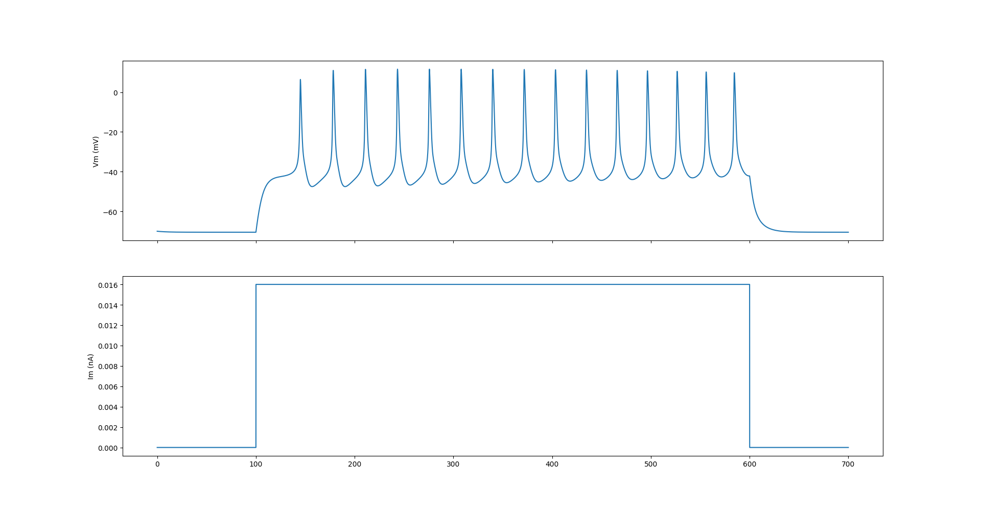
Fig. 72 The membrane potential of the NEURON implementation of the KC cell model with a step current.

We write a quick simulation to reproduce these using our NeuroML model:

def step_current_omv_kc():
    """Create a step current simulation OMV LEMS file"""
    # read the cell file, modify it, write a new one
    netdoc = read_neuroml2_file("KC.cell.nml")
    kc_cell = netdoc.cells[0]
    net = netdoc.add(neuroml.Network, id="KC_net", validate=False)
    pop = net.add(neuroml.Population, id="KC_pop", component=kc_cell.id, size=1)

    # should be same as test_kc.py
    pg = netdoc.add(
        neuroml.PulseGenerator(
            id="pg", delay="100ms", duration="500ms",
            amplitude="16pA"
        )
    )

    # Add these to cells
    input_list = net.add(
        neuroml.InputList(id="input_list", component=pg.id, populations=pop.id)
    )
    aninput = input_list.add(
        neuroml.Input(
            id="0",
            target="../%s[0]" % (pop.id),
            destination="synapses",
            segment_id="0",
        )
    )
    write_neuroml2_file(netdoc, "KC.net.nml")

    generate_lems_file_for_neuroml(
        sim_id="KC_step_test",
        target=net.id,
        neuroml_file="KC.net.nml",
        duration="700ms",
        dt="0.01ms",
        lems_file_name="LEMS_KC_step_test.xml",
        nml_doc=netdoc,
        gen_spike_saves_for_all_somas=True,
        target_dir=".",
        gen_saves_for_quantities={
            "k.dat": ["KC_pop[0]/biophys/membraneProperties/kv/iDensity"]
        },
        copy_neuroml=False
    )

    data = run_lems_with_jneuroml_neuron(
        "LEMS_KC_step_test.xml", load_saved_data=True, compile_mods=True
    )

    generate_plot(
        xvalues=[data["t"]],
        yvalues=[data["KC_pop[0]/v"]],
        title="Membrane potential: KC",
    )

This will generate graphs of the KC’s membrane potential.

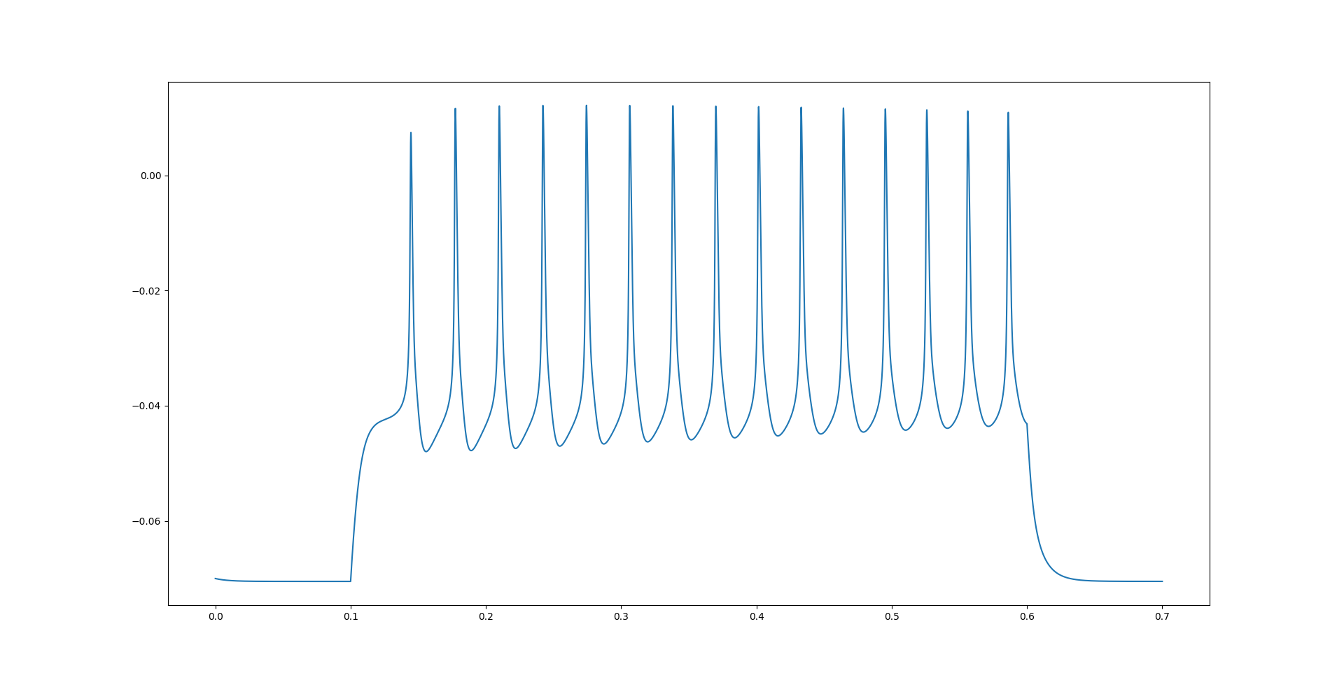
Fig. 73 The membrane potential of the NeuroML implementation of the KC cell model with a step current.

As we can see, the membrane potentials look very similar. In the next page, we will also set up some more validation tests to better verify that the NEURON and NeuroML implementations produce the same dynamics.

Since this writes a LEMS simulation file also, we can also run the LEMS file directly for later verification:

pynml LEMS_KC_step_test.xml -neuron -nogui