Interactive single Izhikevich neuron NeuroML example#
To run this interactive Jupyter Notebook when viewing the online NeuroML documentation (e.g. via Binder or Google Colab), please click on the rocket icon 🚀 in the top panel. For more information, please see how to use this documentation.
This notebook creates a simple model in NeuroML version 2. It adds a simple spiking neuron model to a population and then the population to a network. Then we create a LEMS simulation file to specify how to to a simulate the model, and finally we execute it using jNeuroML. The results of that simulation are plotted below.
See also a more detailed introduction to NeuroML and LEMS using this example.
1) Initial setup and library installs#
Please uncomment the line below if you use the Google Colab (it does not include these packages by default).
#%pip install pyneuroml neuromllite NEURON
from neuroml import NeuroMLDocument
import neuroml.writers as writers
from neuroml.utils import component_factory
from neuroml.utils import validate_neuroml2
from pyneuroml import pynml
from pyneuroml.lems import LEMSSimulation
import numpy as np
2) Declaring the NeuroML model#
Create a NeuroML document#
This is the container document to which the cells and the network will be added.
nml_doc = component_factory(NeuroMLDocument, id="IzhSingleNeuron")
Define the Izhikevich cell and add it to the model#
The Izhikevich model is a simple, 2 variable neuron model exhibiting a range of neurophysiologically realistic spiking behaviours depending on the parameters given. We use the izhikevich2007cell version here.
izh0 = nml_doc.add(
    "Izhikevich2007Cell",
    id="izh2007RS0", v0="-60mV", C="100pF", k="0.7nS_per_mV", vr="-60mV",
    vt="-40mV", vpeak="35mV", a="0.03per_ms", b="-2nS", c="-50.0mV", d="100pA")
Create a network and add it to the model#
We add a network to the document created above.
net = nml_doc.add("Network", id="IzNet", validate=False)
Create a population of defined cells and add it to the model#
A population of size 1 of these cells is created and then added to the network.
size0 = 1
pop0 = net.add("Population", id="IzhPop0", component=izh0.id, size=size0)
Define an external stimulus and add it to the model#
On its own the cell will not spike, so we add a small current to it in the form of a pulse generator which will apply a square pulse of current.
pg = nml_doc.add(
    "PulseGenerator",
    id="pulseGen_%i" % 0, delay="0ms", duration="1000ms",
    amplitude="0.07 nA"
)
exp_input = net.add("ExplicitInput", target="%s[%i]" % (pop0.id, 0), input=pg.id)
3) Write, print and validate the generated file#
Write the NeuroML model to a file#
nml_file = 'izhikevich2007_single_cell_network.nml'
writers.NeuroMLWriter.write(nml_doc, nml_file)
print("Written network file to: " + nml_file)
Written network file to: izhikevich2007_single_cell_network.nml
Print out the file#
Here we print the XML for the saved NeuroML file.
with open(nml_file) as f:
   print(f.read())
<neuroml xmlns="http://www.neuroml.org/schema/neuroml2"  xmlns:xs="http://www.w3.org/2001/XMLSchema" xmlns:xsi="http://www.w3.org/2001/XMLSchema-instance" xsi:schemaLocation="http://www.neuroml.org/schema/neuroml2 https://raw.github.com/NeuroML/NeuroML2/development/Schemas/NeuroML2/NeuroML_v2.3.xsd" id="IzhSingleNeuron">
    <izhikevich2007Cell id="izh2007RS0" C="100pF" v0="-60mV" k="0.7nS_per_mV" vr="-60mV" vt="-40mV" vpeak="35mV" a="0.03per_ms" b="-2nS" c="-50.0mV" d="100pA"/>
    <pulseGenerator id="pulseGen_0" delay="0ms" duration="1000ms" amplitude="0.07 nA"/>
    <network id="IzNet">
        <population id="IzhPop0" component="izh2007RS0" size="1"/>
        <explicitInput target="IzhPop0[0]" input="pulseGen_0"/>
    </network>
</neuroml>
Validate the NeuroML model#
validate_neuroml2(nml_file)
It's valid!
4) Simulating the model#
Create a simulation instance of the model#
The NeuroML file does not contain any information on how long to simulate the model for or what to save etc. For this we will need a LEMS simulation file.
simulation_id = "example-single-izhikevich2007cell-sim"
simulation = LEMSSimulation(sim_id=simulation_id,
                            duration=1000, dt=0.1, simulation_seed=123)
simulation.assign_simulation_target(net.id)
simulation.include_neuroml2_file(nml_file)
pyNeuroML >>> INFO - Loading NeuroML2 file: /Users/padraig/git/Documentation/source/Userdocs/NML2_examples/izhikevich2007_single_cell_network.nml
Define the output file to store simulation outputs#
Here, we record the neuron’s membrane potential to the specified data file.
simulation.create_output_file(
    "output0", "%s.v.dat" % simulation_id
)
simulation.add_column_to_output_file("output0", 'IzhPop0[0]', 'IzhPop0[0]/v')
Save the simulation to a file#
lems_simulation_file = simulation.save_to_file()
with open(lems_simulation_file) as f:
   print(f.read())
<Lems>

    <!--

        This LEMS file has been automatically generated using PyNeuroML v1.1.10 (libNeuroML v0.5.8)

     -->

    <!-- Specify which component to run -->
    <Target component="example-single-izhikevich2007cell-sim"/>

    <!-- Include core NeuroML2 ComponentType definitions -->
    <Include file="Cells.xml"/>
    <Include file="Networks.xml"/>
    <Include file="Simulation.xml"/>

    <Include file="izhikevich2007_single_cell_network.nml"/>

    <Simulation id="example-single-izhikevich2007cell-sim" length="1000ms" step="0.1ms" target="IzNet" seed="123">  <!-- Note seed: ensures same random numbers used every run -->
        <OutputFile id="output0" fileName="example-single-izhikevich2007cell-sim.v.dat">
            <OutputColumn id="IzhPop0[0]" quantity="IzhPop0[0]/v"/>
        </OutputFile>

    </Simulation>

</Lems>
Run the simulation using the jNeuroML simulator#
pynml.run_lems_with_jneuroml(
    lems_simulation_file, max_memory="2G", nogui=True, plot=False
)
pyNeuroML >>> INFO - Loading LEMS file: LEMS_example-single-izhikevich2007cell-sim.xml and running with jNeuroML
pyNeuroML >>> INFO - Executing: (java -Xmx2G  -Djava.awt.headless=true -jar  "/opt/homebrew/anaconda3/envs/py39n/lib/python3.9/site-packages/pyneuroml/lib/jNeuroML-0.13.0-jar-with-dependencies.jar"  LEMS_example-single-izhikevich2007cell-sim.xml  -nogui -I '') in directory: .
pyNeuroML >>> INFO - Command completed successfully!
True
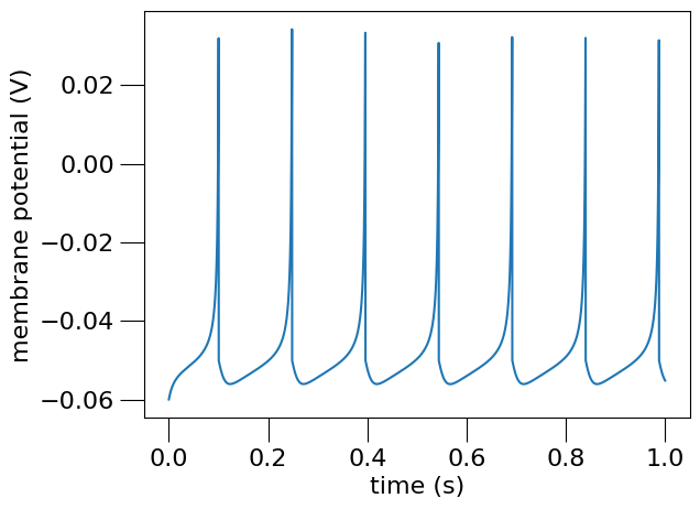
Plot the recorded data#
# Load the data from the file and plot the graph for the membrane potential
# using the pynml generate_plot utility function.
data_array = np.loadtxt("%s.v.dat" % simulation_id)
pynml.generate_plot(
    [data_array[:, 0]], [data_array[:, 1]],
    "Membrane potential", show_plot_already=True,
    xaxis="time (s)", yaxis="membrane potential (V)",
    save_figure_to="SingleNeuron.png"

)
pyNeuroML >>> INFO - Generating plot: Membrane potential
pyNeuroML >>> INFO - Saving image to /Users/padraig/git/Documentation/source/Userdocs/NML2_examples/SingleNeuron.png of plot: Membrane potential
pyNeuroML >>> INFO - Saved image to SingleNeuron.png of plot: Membrane potential

<Axes: xlabel='time (s)', ylabel='membrane potential (V)'>