Simulating a multi compartment OLM neuron#
In this section we will model and simulate a multi-compartment Oriens-lacunosum moleculare (OLM) interneuron cell from the rodent hippocampal CA1 network model developed by Bezaire et al. ([BRB+16]). The complete network model can be seen here on GitHub, and here on Open Source Brain.
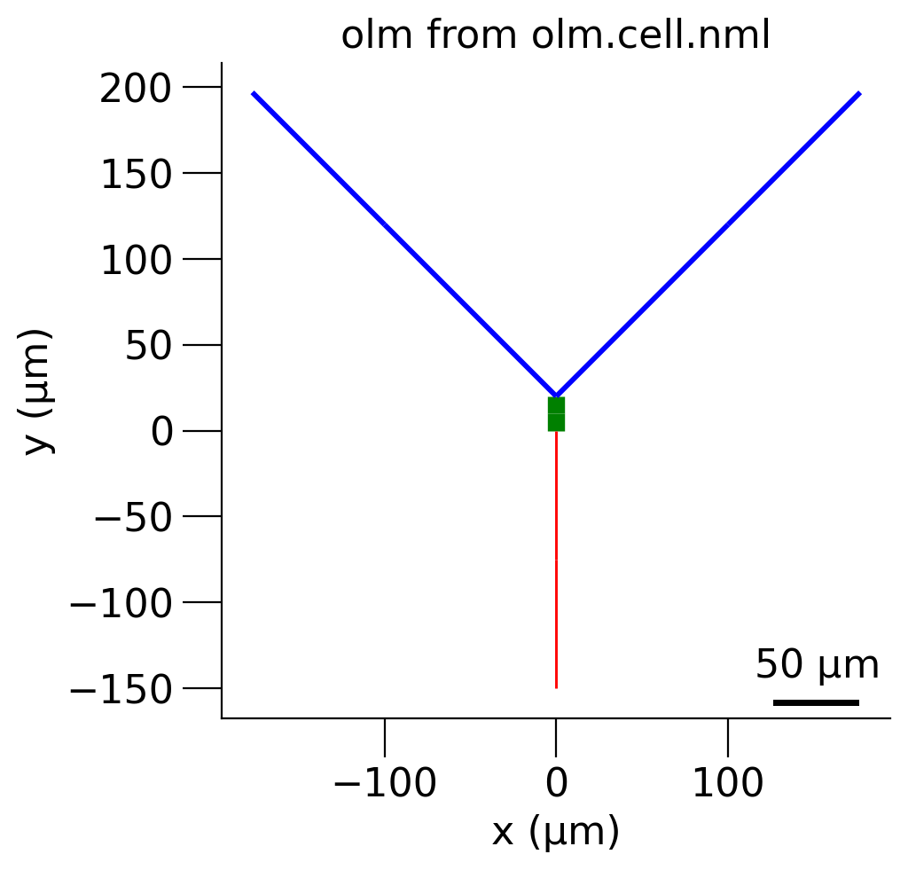
Fig. 22 Morphology of OLM cell in xy plane#
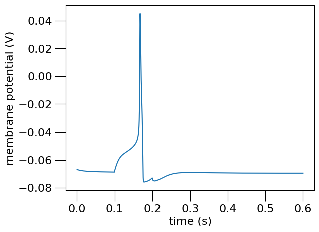
Fig. 23 Membrane potential of the simulated OLM cell at the soma.#
This plot, saved as olm_example_sim_seg0_soma0-v.png is generated using the following Python NeuroML script:
#!/usr/bin/env python3
"""
Multi-compartmental OLM cell example

File: olm-example.py

Copyright 2023 NeuroML contributors
Authors: Padraig Gleeson, Ankur Sinha
"""

import neuroml
from neuroml import NeuroMLDocument
from neuroml.utils import component_factory
from pyneuroml import pynml
from pyneuroml.lems import LEMSSimulation
from pyneuroml.plot.PlotMorphology import plot_2D
import numpy as np


def main():
    """Main function

    Include the NeuroML model into a LEMS simulation file, run it, plot some
    data.
    """
    # Simulation bits
    sim_id = "olm_example_sim"
    simulation = LEMSSimulation(sim_id=sim_id, duration=600, dt=0.01, simulation_seed=123)
    # Include the NeuroML model file
    simulation.include_neuroml2_file(create_olm_network())
    # Assign target for the simulation
    simulation.assign_simulation_target("single_olm_cell_network")

    # Recording information from the simulation
    simulation.create_output_file(id="output0", file_name=sim_id + ".dat")
    simulation.add_column_to_output_file("output0", column_id="pop0_0_v", quantity="pop0[0]/v")
    simulation.add_column_to_output_file("output0",
                                         column_id="pop0_0_v_Seg0_soma_0",
                                         quantity="pop0/0/olm/0/v")
    simulation.add_column_to_output_file("output0",
                                         column_id="pop0_0_v_Seg1_soma_0",
                                         quantity="pop0/0/olm/1/v")
    simulation.add_column_to_output_file("output0",
                                         column_id="pop0_0_v_Seg0_axon_0",
                                         quantity="pop0/0/olm/2/v")
    simulation.add_column_to_output_file("output0",
                                         column_id="pop0_0_v_Seg1_axon_0",
                                         quantity="pop0/0/olm/3/v")
    simulation.add_column_to_output_file("output0",
                                         column_id="pop0_0_v_Seg0_dend_0",
                                         quantity="pop0/0/olm/4/v")
    simulation.add_column_to_output_file("output0",
                                         column_id="pop0_0_v_Seg1_dend_0",
                                         quantity="pop0/0/olm/6/v")
    simulation.add_column_to_output_file("output0",
                                         column_id="pop0_0_v_Seg0_dend_1",
                                         quantity="pop0/0/olm/5/v")
    simulation.add_column_to_output_file("output0",
                                         column_id="pop0_0_v_Seg1_dend_1",
                                         quantity="pop0/0/olm/7/v")
    # Save LEMS simulation to file
    sim_file = simulation.save_to_file()

    # Run the simulation using the NEURON simulator
    pynml.run_lems_with_jneuroml_neuron(sim_file, max_memory="2G", nogui=True,
                                        plot=False, skip_run=False)
    # Plot the data
    plot_data(sim_id)


def plot_data(sim_id):
    """Plot the sim data.

    Load the data from the file and plot the graph for the membrane potential
    using the pynml generate_plot utility function.

    :sim_id: ID of simulaton

    """
    data_array = np.loadtxt(sim_id + ".dat")
    pynml.generate_plot([data_array[:, 0]], [data_array[:, 1]], "Membrane potential (soma seg 0)", show_plot_already=False, save_figure_to=sim_id + "_seg0_soma0-v.png", xaxis="time (s)", yaxis="membrane potential (V)")
    pynml.generate_plot([data_array[:, 0]], [data_array[:, 2]], "Membrane potential (soma seg 1)", show_plot_already=False, save_figure_to=sim_id + "_seg1_soma0-v.png", xaxis="time (s)", yaxis="membrane potential (V)")
    pynml.generate_plot([data_array[:, 0]], [data_array[:, 3]], "Membrane potential (axon seg 0)", show_plot_already=False, save_figure_to=sim_id + "_seg0_axon0-v.png", xaxis="time (s)", yaxis="membrane potential (V)")
    pynml.generate_plot([data_array[:, 0]], [data_array[:, 4]], "Membrane potential (axon seg 1)", show_plot_already=False, save_figure_to=sim_id + "_seg1_axon0-v.png", xaxis="time (s)", yaxis="membrane potential (V)")


def create_olm_network():
    """Create the network

    :returns: name of network nml file
    """
    net_doc = NeuroMLDocument(id="network",
                              notes="OLM cell network")
    net_doc_fn = "olm_example_net.nml"
    net_doc.add("IncludeType", href=create_olm_cell())
    net = net_doc.add("Network", id="single_olm_cell_network", validate=False)
    # Create a population: convenient to create many cells of the same type
    pop = net.add("Population", id="pop0", notes="A population for our cell",
                  component="olm", size=1, type="populationList",
                  validate=False)
    pop.add("Instance", id=0, location=component_factory("Location", x=0., y=0., z=0.))
    # Input
    net_doc.add("PulseGenerator", id="pg_olm", notes="Simple pulse generator", delay="100ms", duration="100ms", amplitude="0.08nA")

    net.add("ExplicitInput", target="pop0[0]", input="pg_olm")

    pynml.write_neuroml2_file(nml2_doc=net_doc, nml2_file_name=net_doc_fn, validate=True)
    return net_doc_fn


def create_olm_cell():
    """Create the complete cell.

    :returns: cell object
    """
    nml_cell_doc = component_factory("NeuroMLDocument", id="oml_cell")
    cell = nml_cell_doc.add("Cell", id="olm", neuro_lex_id="NLXCELL:091206")  # type neuroml.Cell
    nml_cell_file = cell.id + ".cell.nml"

    cell.summary()
    cell.info(show_contents=True)
    cell.morphology.info(show_contents=True)

    # Add two soma segments to an unbranched segment group
    cell.add_unbranched_segment_group("soma_0")
    diam = 10.0
    soma_0 = cell.add_segment(
        prox=[0.0, 0.0, 0.0, diam],
        dist=[0.0, 10., 0.0, diam],
        name="Seg0_soma_0",
        group_id="soma_0",
        seg_type="soma"
    )

    soma_1 = cell.add_segment(
        prox=None,
        dist=[0.0, 10. + 10., 0.0, diam],
        name="Seg1_soma_0",
        parent=soma_0,
        group_id="soma_0",
        seg_type="soma"
    )

    # Add axon segments
    diam = 1.5
    cell.add_unbranched_segments(
        [
            [0.0, 0.0, 0.0, diam],
            [0.0, -75, 0.0, diam],
            [0.0, -150, 0.0, diam],
        ],
        parent=soma_0,
        fraction_along=0.0,
        group_id="axon_0",
        seg_type="axon"
    )

    # Add 2 dendrite segments, using the branching utility function

    diam = 3.0
    cell.add_unbranched_segments(
        [
            [0.0, 20.0, 0.0, diam],
            [100, 120, 0.0, diam],
            [177, 197, 0.0, diam],
        ],
        parent=soma_1,
        fraction_along=1.0,
        group_id="dend_0",
        seg_type="dendrite"
    )

    cell.add_unbranched_segments(
        [
            [0.0, 20.0, 0.0, diam],
            [-100, 120, 0.0, diam],
            [-177, 197, 0.0, diam],
        ],
        parent=soma_1,
        fraction_along=1.0,
        group_id="dend_1",
        seg_type="dendrite"
    )

    # color groups for morphology plots
    den_seg_group = cell.get_segment_group("dendrite_group")
    den_seg_group.add("Property", tag="color", value="0.8 0 0")

    ax_seg_group = cell.get_segment_group("axon_group")
    ax_seg_group.add("Property", tag="color", value="0 0.8 0")

    soma_seg_group = cell.get_segment_group("soma_group")
    soma_seg_group.add("Property", tag="color", value="0 0 0.8")

    # Other cell properties
    cell.set_init_memb_potential("-67mV")
    cell.set_resistivity("0.15 kohm_cm")
    cell.set_specific_capacitance("1.3 uF_per_cm2")
    cell.set_spike_thresh("-20 mV")

    # channels
    # leak
    cell.add_channel_density(nml_cell_doc,
                             cd_id="leak_all",
                             cond_density="0.01 mS_per_cm2",
                             ion_channel="leak_chan",
                             ion_chan_def_file="olm-example/leak_chan.channel.nml",
                             erev="-67mV",
                             ion="non_specific")
    # HCNolm_soma
    cell.add_channel_density(nml_cell_doc,
                             cd_id="HCNolm_soma",
                             cond_density="0.5 mS_per_cm2",
                             ion_channel="HCNolm",
                             ion_chan_def_file="olm-example/HCNolm.channel.nml",
                             erev="-32.9mV",
                             ion="h",
                             group_id="soma_group")
    # Kdrfast_soma
    cell.add_channel_density(nml_cell_doc,
                             cd_id="Kdrfast_soma",
                             cond_density="73.37 mS_per_cm2",
                             ion_channel="Kdrfast",
                             ion_chan_def_file="olm-example/Kdrfast.channel.nml",
                             erev="-77mV",
                             ion="k",
                             group_id="soma_group")
    # Kdrfast_dendrite
    cell.add_channel_density(nml_cell_doc,
                             cd_id="Kdrfast_dendrite",
                             cond_density="105.8 mS_per_cm2",
                             ion_channel="Kdrfast",
                             ion_chan_def_file="olm-example/Kdrfast.channel.nml",
                             erev="-77mV",
                             ion="k",
                             group_id="dendrite_group")
    # Kdrfast_axon
    cell.add_channel_density(nml_cell_doc,
                             cd_id="Kdrfast_axon",
                             cond_density="117.392 mS_per_cm2",
                             ion_channel="Kdrfast",
                             ion_chan_def_file="olm-example/Kdrfast.channel.nml",
                             erev="-77mV",
                             ion="k",
                             group_id="axon_group")
    # KvAolm_soma
    cell.add_channel_density(nml_cell_doc,
                             cd_id="KvAolm_soma",
                             cond_density="4.95 mS_per_cm2",
                             ion_channel="KvAolm",
                             ion_chan_def_file="olm-example/KvAolm.channel.nml",
                             erev="-77mV",
                             ion="k",
                             group_id="soma_group")
    # KvAolm_dendrite
    cell.add_channel_density(nml_cell_doc,
                             cd_id="KvAolm_dendrite",
                             cond_density="2.8 mS_per_cm2",
                             ion_channel="KvAolm",
                             ion_chan_def_file="olm-example/KvAolm.channel.nml",
                             erev="-77mV",
                             ion="k",
                             group_id="dendrite_group")
    # Nav_soma
    cell.add_channel_density(nml_cell_doc,
                             cd_id="Nav_soma",
                             cond_density="10.7 mS_per_cm2",
                             ion_channel="Nav",
                             ion_chan_def_file="olm-example/Nav.channel.nml",
                             erev="50mV",
                             ion="na",
                             group_id="soma_group")
    # Nav_dendrite
    cell.add_channel_density(nml_cell_doc,
                             cd_id="Nav_dendrite",
                             cond_density="23.4 mS_per_cm2",
                             ion_channel="Nav",
                             ion_chan_def_file="olm-example/Nav.channel.nml",
                             erev="50mV",
                             ion="na",
                             group_id="dendrite_group")
    # Nav_axon
    cell.add_channel_density(nml_cell_doc,
                             cd_id="Nav_axon",
                             cond_density="17.12 mS_per_cm2",
                             ion_channel="Nav",
                             ion_chan_def_file="olm-example/Nav.channel.nml",
                             erev="50mV",
                             ion="na",
                             group_id="axon_group")

    cell.optimise_segment_groups()
    cell.validate(recursive=True)
    pynml.write_neuroml2_file(nml_cell_doc, nml_cell_file, True, True)
    plot_2D(nml_cell_file, plane2d="xy", nogui=True,
            save_to_file="olm.cell.xy.png")
    return nml_cell_file


if __name__ == "__main__":
    main()
Declaring the model in NeuroML#
Similar to previous examples, we will first declare the model, visualise it, and then simulate it. The OLM model is slightly more complex than the HH neuron model we had worked with in the previous tutorial since it includes multiple compartments. However, where we had declared the ion-channels ourselves in the previous example, here will will not do so. We will include channels that have been pre-defined in NeuroML to demonstrate how components defined in NeuroML can be easily re-used in models.
We will follow the same method as before. We will first define the cell, create a network with one instance of the cell, and then simulate it to record and plot the membrane potential from different segments.
Declaring the cell#
To keep our Python script modularised, we start constructing our cell in a separate function.
def create_olm_cell():
    """Create the complete cell.

    :returns: cell object
    """
    nml_cell_doc = component_factory("NeuroMLDocument", id="oml_cell")
    cell = nml_cell_doc.add("Cell", id="olm", neuro_lex_id="NLXCELL:091206")  # type neuroml.Cell
    nml_cell_file = cell.id + ".cell.nml"

    cell.summary()
    cell.info(show_contents=True)
    cell.morphology.info(show_contents=True)

    # Add two soma segments to an unbranched segment group
    cell.add_unbranched_segment_group("soma_0")
    diam = 10.0
    soma_0 = cell.add_segment(
        prox=[0.0, 0.0, 0.0, diam],
        dist=[0.0, 10., 0.0, diam],
        name="Seg0_soma_0",
        group_id="soma_0",
        seg_type="soma"
    )

    soma_1 = cell.add_segment(
        prox=None,
        dist=[0.0, 10. + 10., 0.0, diam],
        name="Seg1_soma_0",
        parent=soma_0,
        group_id="soma_0",
        seg_type="soma"
    )

    # Add axon segments
    diam = 1.5
    cell.add_unbranched_segments(
        [
            [0.0, 0.0, 0.0, diam],
            [0.0, -75, 0.0, diam],
            [0.0, -150, 0.0, diam],
        ],
        parent=soma_0,
        fraction_along=0.0,
        group_id="axon_0",
        seg_type="axon"
    )

    # Add 2 dendrite segments, using the branching utility function

    diam = 3.0
    cell.add_unbranched_segments(
        [
            [0.0, 20.0, 0.0, diam],
            [100, 120, 0.0, diam],
            [177, 197, 0.0, diam],
        ],
        parent=soma_1,
        fraction_along=1.0,
        group_id="dend_0",
        seg_type="dendrite"
    )

    cell.add_unbranched_segments(
        [
            [0.0, 20.0, 0.0, diam],
            [-100, 120, 0.0, diam],
            [-177, 197, 0.0, diam],
        ],
        parent=soma_1,
        fraction_along=1.0,
        group_id="dend_1",
        seg_type="dendrite"
    )

    # color groups for morphology plots
    den_seg_group = cell.get_segment_group("dendrite_group")
    den_seg_group.add("Property", tag="color", value="0.8 0 0")

    ax_seg_group = cell.get_segment_group("axon_group")
    ax_seg_group.add("Property", tag="color", value="0 0.8 0")

    soma_seg_group = cell.get_segment_group("soma_group")
    soma_seg_group.add("Property", tag="color", value="0 0 0.8")

    # Other cell properties
    cell.set_init_memb_potential("-67mV")
    cell.set_resistivity("0.15 kohm_cm")
    cell.set_specific_capacitance("1.3 uF_per_cm2")
    cell.set_spike_thresh("-20 mV")

    # channels
    # leak
    cell.add_channel_density(nml_cell_doc,
                             cd_id="leak_all",
                             cond_density="0.01 mS_per_cm2",
                             ion_channel="leak_chan",
                             ion_chan_def_file="olm-example/leak_chan.channel.nml",
                             erev="-67mV",
                             ion="non_specific")
    # HCNolm_soma
    cell.add_channel_density(nml_cell_doc,
                             cd_id="HCNolm_soma",
                             cond_density="0.5 mS_per_cm2",
                             ion_channel="HCNolm",
                             ion_chan_def_file="olm-example/HCNolm.channel.nml",
                             erev="-32.9mV",
                             ion="h",
                             group_id="soma_group")
    # Kdrfast_soma
    cell.add_channel_density(nml_cell_doc,
                             cd_id="Kdrfast_soma",
                             cond_density="73.37 mS_per_cm2",
                             ion_channel="Kdrfast",
                             ion_chan_def_file="olm-example/Kdrfast.channel.nml",
                             erev="-77mV",
                             ion="k",
                             group_id="soma_group")
    # Kdrfast_dendrite
    cell.add_channel_density(nml_cell_doc,
                             cd_id="Kdrfast_dendrite",
                             cond_density="105.8 mS_per_cm2",
                             ion_channel="Kdrfast",
                             ion_chan_def_file="olm-example/Kdrfast.channel.nml",
                             erev="-77mV",
                             ion="k",
                             group_id="dendrite_group")
    # Kdrfast_axon
    cell.add_channel_density(nml_cell_doc,
                             cd_id="Kdrfast_axon",
                             cond_density="117.392 mS_per_cm2",
                             ion_channel="Kdrfast",
                             ion_chan_def_file="olm-example/Kdrfast.channel.nml",
                             erev="-77mV",
                             ion="k",
                             group_id="axon_group")
    # KvAolm_soma
    cell.add_channel_density(nml_cell_doc,
                             cd_id="KvAolm_soma",
                             cond_density="4.95 mS_per_cm2",
                             ion_channel="KvAolm",
                             ion_chan_def_file="olm-example/KvAolm.channel.nml",
                             erev="-77mV",
                             ion="k",
                             group_id="soma_group")
    # KvAolm_dendrite
    cell.add_channel_density(nml_cell_doc,
                             cd_id="KvAolm_dendrite",
                             cond_density="2.8 mS_per_cm2",
                             ion_channel="KvAolm",
                             ion_chan_def_file="olm-example/KvAolm.channel.nml",
                             erev="-77mV",
                             ion="k",
                             group_id="dendrite_group")
    # Nav_soma
    cell.add_channel_density(nml_cell_doc,
                             cd_id="Nav_soma",
                             cond_density="10.7 mS_per_cm2",
                             ion_channel="Nav",
                             ion_chan_def_file="olm-example/Nav.channel.nml",
                             erev="50mV",
                             ion="na",
                             group_id="soma_group")
    # Nav_dendrite
    cell.add_channel_density(nml_cell_doc,
                             cd_id="Nav_dendrite",
                             cond_density="23.4 mS_per_cm2",
                             ion_channel="Nav",
                             ion_chan_def_file="olm-example/Nav.channel.nml",
                             erev="50mV",
                             ion="na",
                             group_id="dendrite_group")
    # Nav_axon
    cell.add_channel_density(nml_cell_doc,
                             cd_id="Nav_axon",
                             cond_density="17.12 mS_per_cm2",
                             ion_channel="Nav",
                             ion_chan_def_file="olm-example/Nav.channel.nml",
                             erev="50mV",
                             ion="na",
                             group_id="axon_group")
Let us walk through this function:
    nml_cell_doc = component_factory("NeuroMLDocument", id="oml_cell")
    cell = nml_cell_doc.add("Cell", id="olm", neuro_lex_id="NLXCELL:091206")  # type neuroml.Cell
    nml_cell_file = cell.id + ".cell.nml"

    cell.summary()
    cell.info(show_contents=True)
    cell.morphology.info(show_contents=True)
We create a new model document that will hold the cell model.
Then, we create and add a new Cell using the add method to the document.
We also provide a neuro_lex_id here, which is the NeuroLex ontology identifier.
This allows us to better connect models to biological concepts.
As we have seen in the single Izhikevich neuron example, the add method calls the component_factory to create the component object for us.
For the Cell component type, it does a number of extra things for us to set up, or initialise, the cell.
We have a number of ways of inspecting the cell.
The summary function provides a very short summary of the cell.
This is useful to quickly get a high level overview of it:
>>> cell.summary()
*******************************************************
* Cell: olm
* Notes: None
* Segments: 0
* SegmentGroups: 4
*******************************************************
We can also use the general info function to inspect the cell:
>>> cell.info(show_contents=True)
Cell -- Cell with  **segment** s specified in a  **morphology**  element along with details on its  **biophysicalProperties** . NOTE: this can only be correctly simulated using jLEMS when there is a single segment in the cell, and **v**  of this cell represents the membrane potential in that isopotential segment.

Please see the NeuroML standard schema documentation at https://docs.neuroml.org/Userdocs/NeuroMLv2.html for more information.

Valid members for Cell are:
* biophysical_properties_attr (class: NmlId, Optional)
* morphology (class: Morphology, Optional)
        * Contents ('ids'/<objects>): 'morphology'

* neuro_lex_id (class: NeuroLexId, Optional)
        * Contents ('ids'/<objects>): NLXCELL:091206

* metaid (class: MetaId, Optional)
* biophysical_properties (class: BiophysicalProperties, Optional)
        * Contents ('ids'/<objects>): 'biophys'

* id (class: NmlId, Required)
        * Contents ('ids'/<objects>): olm

* notes (class: xs:string, Optional)
* properties (class: Property, Optional)
* annotation (class: Annotation, Optional)
* morphology_attr (class: NmlId, Optional)
We see the cell already contains biophysical_properties or morphology.
Because these are components of the cell that are expected to be used, these were added automatically for us when the new component was created.
Let us take a look at the morphology of the cell:
>>> cell.morphology.info(show_contents=True)
Morphology -- The collection of  **segment** s which specify the 3D structure of the cell, along with a number of  **segmentGroup** s

Please see the NeuroML standard schema documentation at https://docs.neuroml.org/Userdocs/NeuroMLv2.html for more information.

Valid members for Morphology are:
* segments (class: Segment, Required)
* metaid (class: MetaId, Optional)
* segment_groups (class: SegmentGroup, Optional)
        * Contents ('ids'/<objects>): ['all', 'soma_group', 'axon_group', 'dendrite_group']

* id (class: NmlId, Required)
        * Contents ('ids'/<objects>): morphology

* notes (class: xs:string, Optional)
* properties (class: Property, Optional)
* annotation (class: Annotation, Optional)
We see that there are no segments in the cell because we have not added any.
However, there are already a number of “default” segment groups that were automatically added for us: all, soma_group, axon_group, dendrite_group.
These groups allow us to keep track of all the segments, and of the segments forming the soma, the axon, and the dendrites of the cell respectively.
Take a look at the conventions page for more information on these.
We now have an empty cell.
Since we are building a multi-compartmental cell, we now proceed to define the detailed morphology of the cell.
We do this by adding segments and grouping them in to segment groups.
We can add segments using the add_segment utility function, as we do for the segments forming the soma.
Here, our soma has two segments.
    # Add two soma segments to an unbranched segment group
    cell.add_unbranched_segment_group("soma_0")
    diam = 10.0
    soma_0 = cell.add_segment(
        prox=[0.0, 0.0, 0.0, diam],
        dist=[0.0, 10., 0.0, diam],
        name="Seg0_soma_0",
        group_id="soma_0",
        seg_type="soma"
    )

    soma_1 = cell.add_segment(
        prox=None,
        dist=[0.0, 10. + 10., 0.0, diam],
        name="Seg1_soma_0",
        parent=soma_0,
        group_id="soma_0",
        seg_type="soma"
    )
The utility function takes the dimensions of the segment—it’s proximal and distal co-ordinates and the diameter to create a segment of the provided name. Additionally, since segments need to be contiguous, it makes the first segment the parent of the second, to build a chain. Finally, it places the segment into the specified segment group and the default groups that we also have and adds the segment to the cell’s morphology.
Note that by default, the add_segment function does not know if the segments are contiguous, i.e., that they form an unbranched branch of the cell.
We could have added segments here that do not line up in a chain, when building different parts of a cell for example.
In this case, we know that the two soma segments must be contiguous, and that they are on the same unbranched branch (i.e. a continuous section without any branching points on it), so we create an unbranched segment group first using the add_unbranched_segment_group.
If we were only creating cell morphologies, this would not not matter much. Even if the two segments were not included in a group of unbranched segments, they would still be connected. However, for simulation, simulators such as NEURON need to know which parts of the cell form unbranched sections so that they can apply the cable equation and break them into smaller segments to simulate the electric current through them. (See [CGH+07] for more information on how different simulators simulate cells with detailed morphologies.)
Next, we can call the same functions multiple times to add soma, dendritic, and axonal segments to our cell but this can get quite lengthy.
To easily add unbranched contiguous lists of segments to the cell, we can directly use the add_unbranched_segments utility function.
Here we use it to create an axonal segment group, and two dendritic groups each with two segments.
The first point we provide is the proximal (starting) of the dendrite.
The next two points are the distal (ends) of each segment forming the section.
    # Add axon segments
    diam = 1.5
    cell.add_unbranched_segments(
        [
            [0.0, 0.0, 0.0, diam],
            [0.0, -75, 0.0, diam],
            [0.0, -150, 0.0, diam],
        ],
        parent=soma_0,
        fraction_along=0.0,
        group_id="axon_0",
        seg_type="axon"
    )

    # Add 2 dendrite segments, using the branching utility function

    diam = 3.0
    cell.add_unbranched_segments(
        [
            [0.0, 20.0, 0.0, diam],
            [100, 120, 0.0, diam],
            [177, 197, 0.0, diam],
        ],
        parent=soma_1,
        fraction_along=1.0,
        group_id="dend_0",
        seg_type="dendrite"
    )

    cell.add_unbranched_segments(
        [
            [0.0, 20.0, 0.0, diam],
            [-100, 120, 0.0, diam],
            [-177, 197, 0.0, diam],
        ],
        parent=soma_1,
        fraction_along=1.0,
        group_id="dend_1",
        seg_type="dendrite"
    )
We repeat this process to create more dendritic and axonal sections of contiguous segments.
Finally, we add an extra colour property to the three primary segment groups that can be used when generating morphology graphs:
    # color groups for morphology plots
    den_seg_group = cell.get_segment_group("dendrite_group")
    den_seg_group.add("Property", tag="color", value="0.8 0 0")

    ax_seg_group = cell.get_segment_group("axon_group")
    ax_seg_group.add("Property", tag="color", value="0 0.8 0")

    soma_seg_group = cell.get_segment_group("soma_group")
    soma_seg_group.add("Property", tag="color", value="0 0 0.8")
We have now completed adding the morphological information to our cell. Next, we proceed to our biophysical properties, e.g.:
We use more helpful utility functions to set these values
    # Other cell properties
    cell.set_init_memb_potential("-67mV")
    cell.set_resistivity("0.15 kohm_cm")
    cell.set_specific_capacitance("1.3 uF_per_cm2")
For setting channel densities, we have the add_channel_density function:
    # channels
    # leak
    cell.add_channel_density(nml_cell_doc,
                             cd_id="leak_all",
                             cond_density="0.01 mS_per_cm2",
                             ion_channel="leak_chan",
                             ion_chan_def_file="olm-example/leak_chan.channel.nml",
                             erev="-67mV",
                             ion="non_specific")
    # HCNolm_soma
    cell.add_channel_density(nml_cell_doc,
                             cd_id="HCNolm_soma",
                             cond_density="0.5 mS_per_cm2",
                             ion_channel="HCNolm",
                             ion_chan_def_file="olm-example/HCNolm.channel.nml",
                             erev="-32.9mV",
                             ion="h",
                             group_id="soma_group")
    # Kdrfast_soma
    cell.add_channel_density(nml_cell_doc,
                             cd_id="Kdrfast_soma",
                             cond_density="73.37 mS_per_cm2",
                             ion_channel="Kdrfast",
                             ion_chan_def_file="olm-example/Kdrfast.channel.nml",
                             erev="-77mV",
                             ion="k",
                             group_id="soma_group")
    # Kdrfast_dendrite
    cell.add_channel_density(nml_cell_doc,
                             cd_id="Kdrfast_dendrite",
                             cond_density="105.8 mS_per_cm2",
                             ion_channel="Kdrfast",
                             ion_chan_def_file="olm-example/Kdrfast.channel.nml",
                             erev="-77mV",
                             ion="k",
                             group_id="dendrite_group")
    # Kdrfast_axon
    cell.add_channel_density(nml_cell_doc,
                             cd_id="Kdrfast_axon",
                             cond_density="117.392 mS_per_cm2",
                             ion_channel="Kdrfast",
                             ion_chan_def_file="olm-example/Kdrfast.channel.nml",
                             erev="-77mV",
                             ion="k",
                             group_id="axon_group")
    # KvAolm_soma
    cell.add_channel_density(nml_cell_doc,
                             cd_id="KvAolm_soma",
                             cond_density="4.95 mS_per_cm2",
                             ion_channel="KvAolm",
                             ion_chan_def_file="olm-example/KvAolm.channel.nml",
                             erev="-77mV",
                             ion="k",
                             group_id="soma_group")
    # KvAolm_dendrite
    cell.add_channel_density(nml_cell_doc,
                             cd_id="KvAolm_dendrite",
                             cond_density="2.8 mS_per_cm2",
                             ion_channel="KvAolm",
                             ion_chan_def_file="olm-example/KvAolm.channel.nml",
                             erev="-77mV",
                             ion="k",
                             group_id="dendrite_group")
    # Nav_soma
    cell.add_channel_density(nml_cell_doc,
                             cd_id="Nav_soma",
                             cond_density="10.7 mS_per_cm2",
                             ion_channel="Nav",
                             ion_chan_def_file="olm-example/Nav.channel.nml",
                             erev="50mV",
                             ion="na",
                             group_id="soma_group")
    # Nav_dendrite
    cell.add_channel_density(nml_cell_doc,
                             cd_id="Nav_dendrite",
                             cond_density="23.4 mS_per_cm2",
                             ion_channel="Nav",
                             ion_chan_def_file="olm-example/Nav.channel.nml",
                             erev="50mV",
                             ion="na",
                             group_id="dendrite_group")
    # Nav_axon
    cell.add_channel_density(nml_cell_doc,
                             cd_id="Nav_axon",
                             cond_density="17.12 mS_per_cm2",
                             ion_channel="Nav",
                             ion_chan_def_file="olm-example/Nav.channel.nml",
                             erev="50mV",
                             ion="na",
Note that we are not writing our channel files from scratch here. We are re-using already written NeuroML channel definitions by simply including their NeuroML definition files.
This completes the definition of our cell. We now run the level one validation, write it to a file while also running a complete (level one and level two) validation using pyNeuroML. We also generate the morphology plot shown on the top of this page.
    cell.optimise_segment_groups()
    cell.validate(recursive=True)
    pynml.write_neuroml2_file(nml_cell_doc, nml_cell_file, True, True)
The resulting NeuroML file is:
<neuroml xmlns="http://www.neuroml.org/schema/neuroml2"  xmlns:xs="http://www.w3.org/2001/XMLSchema" xmlns:xsi="http://www.w3.org/2001/XMLSchema-instance" xsi:schemaLocation="http://www.neuroml.org/schema/neuroml2 https://raw.github.com/NeuroML/NeuroML2/development/Schemas/NeuroML2/NeuroML_v2.3.1.xsd" id="oml_cell">
    <include href="olm-example/leak_chan.channel.nml"/>
    <include href="olm-example/HCNolm.channel.nml"/>
    <include href="olm-example/Kdrfast.channel.nml"/>
    <include href="olm-example/KvAolm.channel.nml"/>
    <include href="olm-example/Nav.channel.nml"/>
    <cell id="olm" neuroLexId="NLXCELL:091206">
        <morphology id="morphology">
            <segment id="0" name="Seg0_soma_0">
                <proximal x="0.0" y="0.0" z="0.0" diameter="10.0"/>
                <distal x="0.0" y="10.0" z="0.0" diameter="10.0"/>
            </segment>
            <segment id="1" name="Seg1_soma_0">
                <parent segment="0"/>
                <distal x="0.0" y="20.0" z="0.0" diameter="10.0"/>
            </segment>
            <segment id="2" name="Seg0_axon_0">
                <parent segment="0" fractionAlong="0.0"/>
                <proximal x="0.0" y="0.0" z="0.0" diameter="1.5"/>
                <distal x="0.0" y="-75.0" z="0.0" diameter="1.5"/>
            </segment>
            <segment id="3" name="Seg1_axon_0">
                <parent segment="2"/>
                <proximal x="0.0" y="-75.0" z="0.0" diameter="1.5"/>
                <distal x="0.0" y="-150.0" z="0.0" diameter="1.5"/>
            </segment>
            <segment id="4" name="Seg0_dend_0">
                <parent segment="1"/>
                <proximal x="0.0" y="20.0" z="0.0" diameter="3.0"/>
                <distal x="100.0" y="120.0" z="0.0" diameter="3.0"/>
            </segment>
            <segment id="5" name="Seg1_dend_0">
                <parent segment="4"/>
                <proximal x="100.0" y="120.0" z="0.0" diameter="3.0"/>
                <distal x="177.0" y="197.0" z="0.0" diameter="3.0"/>
            </segment>
            <segment id="6" name="Seg0_dend_1">
                <parent segment="1"/>
                <proximal x="0.0" y="20.0" z="0.0" diameter="3.0"/>
                <distal x="-100.0" y="120.0" z="0.0" diameter="3.0"/>
            </segment>
            <segment id="7" name="Seg1_dend_1">
                <parent segment="6"/>
                <proximal x="-100.0" y="120.0" z="0.0" diameter="3.0"/>
                <distal x="-177.0" y="197.0" z="0.0" diameter="3.0"/>
            </segment>
            <segmentGroup id="soma_0" neuroLexId="sao864921383">
                <member segment="0"/>
                <member segment="1"/>
            </segmentGroup>
            <segmentGroup id="axon_0" neuroLexId="sao864921383">
                <member segment="2"/>
                <member segment="3"/>
            </segmentGroup>
            <segmentGroup id="dend_0" neuroLexId="sao864921383">
                <member segment="4"/>
                <member segment="5"/>
            </segmentGroup>
            <segmentGroup id="dend_1" neuroLexId="sao864921383">
                <member segment="6"/>
                <member segment="7"/>
            </segmentGroup>
            <segmentGroup id="soma_group" neuroLexId="GO:0043025">
                <notes>Default soma segment group for the cell</notes>
                <property tag="color" value="0 0 0.8"/>
                <include segmentGroup="soma_0"/>
            </segmentGroup>
            <segmentGroup id="axon_group" neuroLexId="GO:0030424">
                <notes>Default axon segment group for the cell</notes>
                <property tag="color" value="0 0.8 0"/>
                <include segmentGroup="axon_0"/>
            </segmentGroup>
            <segmentGroup id="dendrite_group" neuroLexId="GO:0030425">
                <notes>Default dendrite segment group for the cell</notes>
                <property tag="color" value="0.8 0 0"/>
                <include segmentGroup="dend_0"/>
                <include segmentGroup="dend_1"/>
            </segmentGroup>
            <segmentGroup id="all">
                <notes>Default segment group for all segments in the cell</notes>
                <include segmentGroup="axon_0"/>
                <include segmentGroup="dend_0"/>
                <include segmentGroup="dend_1"/>
                <include segmentGroup="soma_0"/>
            </segmentGroup>
        </morphology>
        <biophysicalProperties id="biophys">
            <membraneProperties>
                <channelDensity id="leak_all" ionChannel="leak_chan" condDensity="0.01 mS_per_cm2" erev="-67mV" ion="non_specific"/>
                <channelDensity id="HCNolm_soma" ionChannel="HCNolm" condDensity="0.5 mS_per_cm2" erev="-32.9mV" segmentGroup="soma_group" ion="h"/>
                <channelDensity id="Kdrfast_soma" ionChannel="Kdrfast" condDensity="73.37 mS_per_cm2" erev="-77mV" segmentGroup="soma_group" ion="k"/>
                <channelDensity id="Kdrfast_dendrite" ionChannel="Kdrfast" condDensity="105.8 mS_per_cm2" erev="-77mV" segmentGroup="dendrite_group" ion="k"/>
                <channelDensity id="Kdrfast_axon" ionChannel="Kdrfast" condDensity="117.392 mS_per_cm2" erev="-77mV" segmentGroup="axon_group" ion="k"/>
                <channelDensity id="KvAolm_soma" ionChannel="KvAolm" condDensity="4.95 mS_per_cm2" erev="-77mV" segmentGroup="soma_group" ion="k"/>
                <channelDensity id="KvAolm_dendrite" ionChannel="KvAolm" condDensity="2.8 mS_per_cm2" erev="-77mV" segmentGroup="dendrite_group" ion="k"/>
                <channelDensity id="Nav_soma" ionChannel="Nav" condDensity="10.7 mS_per_cm2" erev="50mV" segmentGroup="soma_group" ion="na"/>
                <channelDensity id="Nav_dendrite" ionChannel="Nav" condDensity="23.4 mS_per_cm2" erev="50mV" segmentGroup="dendrite_group" ion="na"/>
                <channelDensity id="Nav_axon" ionChannel="Nav" condDensity="17.12 mS_per_cm2" erev="50mV" segmentGroup="axon_group" ion="na"/>
                <spikeThresh value="-20 mV"/>
                <specificCapacitance value="1.3 uF_per_cm2"/>
                <initMembPotential value="-67mV"/>
            </membraneProperties>
            <intracellularProperties>
                <resistivity value="0.15 kohm_cm"/>
            </intracellularProperties>
        </biophysicalProperties>
    </cell>
</neuroml>
We can now already inspect our cell using the NeuroML tools.
We have already generated the morphology plot in our script, but we can also do it using pynml:
pynml -png olm.cell.png
...
pyNeuroML >>> Writing to: /home/asinha/Documents/02_Code/00_mine/2020-OSB/NeuroML-Documentation/source/Userdocs/NML2_examples/olm.cell.png
This gives us a figure of the morphology of our cell, similar to the one we’ve already generated:
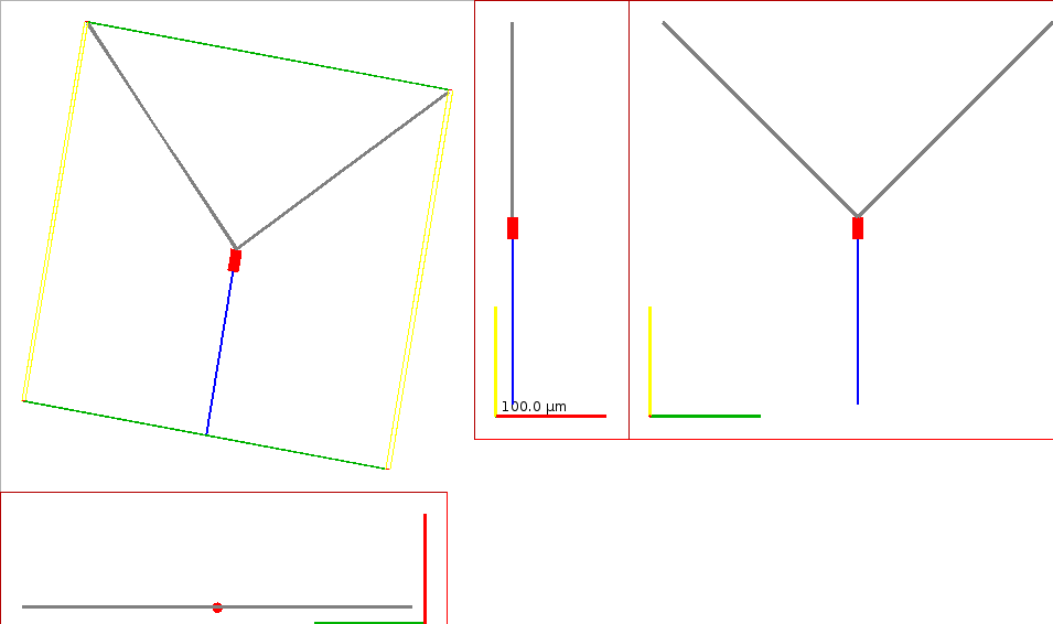
Fig. 24 Figure showing the morphology of the OLM cell generated from the NeuroML definition.#
Declaring the network#
We now use our cell in a network. Similar to our previous example, we are going to only create a network with one cell, and an explicit input to the cell:
def create_olm_network():
    """Create the network

    :returns: name of network nml file
    """
    net_doc = NeuroMLDocument(id="network",
                              notes="OLM cell network")
    net_doc_fn = "olm_example_net.nml"
    net_doc.add("IncludeType", href=create_olm_cell())
    net = net_doc.add("Network", id="single_olm_cell_network", validate=False)
    # Create a population: convenient to create many cells of the same type
    pop = net.add("Population", id="pop0", notes="A population for our cell",
                  component="olm", size=1, type="populationList",
                  validate=False)
    pop.add("Instance", id=0, location=component_factory("Location", x=0., y=0., z=0.))
    # Input
    net_doc.add("PulseGenerator", id="pg_olm", notes="Simple pulse generator", delay="100ms", duration="100ms", amplitude="0.08nA")

    net.add("ExplicitInput", target="pop0[0]", input="pg_olm")

    pynml.write_neuroml2_file(nml2_doc=net_doc, nml2_file_name=net_doc_fn, validate=True)
    return net_doc_fn
We start in the same way, by creating a new NeuroML document and including our cell file into it.
We then create a population comprising of a single cell.
We create a pulse generator as an explicit input, which targets our population.
Note that as the schema documentation for ExplicitInput notes, any current source (any component that extends basePointCurrent) can be used as an ExplicitInput.
We add all of these to the network and save (and validate) our network file. The NeuroML file generated is below:
<neuroml xmlns="http://www.neuroml.org/schema/neuroml2"  xmlns:xs="http://www.w3.org/2001/XMLSchema" xmlns:xsi="http://www.w3.org/2001/XMLSchema-instance" xsi:schemaLocation="http://www.neuroml.org/schema/neuroml2 https://raw.github.com/NeuroML/NeuroML2/development/Schemas/NeuroML2/NeuroML_v2.3.1.xsd" id="network">
    <notes>OLM cell network</notes>
    <include href="olm.cell.nml"/>
    <pulseGenerator id="pg_olm" delay="100ms" duration="100ms" amplitude="0.08nA">
        <notes>Simple pulse generator</notes>
    </pulseGenerator>
    <network id="single_olm_cell_network">
        <population id="pop0" component="olm" size="1" type="populationList">
            <notes>A population for our cell</notes>
            <instance id="0">
                <location x="0.0" y="0.0" z="0.0"/>
            </instance>
        </population>
        <explicitInput target="pop0[0]" input="pg_olm"/>
    </network>
</neuroml>
The generated NeuroML model#
Before we look at simulating the model, we can inspect our model to check for correctness. All our NeuroML files were validated when they were created already, so we do not need to run this step again. However, if required, this can be easily done:
pynml -validate olm*nml
Next, we can visualise our model using the information noted in the visualising NeuroML models page (including the -v verbose option for more information on the cell):
pynml-summary olm_example_net.nml -v
*******************************************************
* NeuroMLDocument: network
*
*  ComponentType: ['Bezaire_HCNolm_tau', 'Bezaire_Kdrfast_betaq', 'Bezaire_KvAolm_taub', 'Bezaire_Nav_alphah']
*  IonChannel: ['HCNolm', 'Kdrfast', 'KvAolm', 'Nav', 'leak_chan']
*  PulseGenerator: ['pg_olm']
*
*  Cell: olm
*    <Segment|0|Seg0_soma_0>
*      Parent segment: None (root segment)
*      (0.0, 0.0, 0.0), diam 10.0um -> (0.0, 10.0, 0.0), diam 10.0um; seg length: 10.0 um
*      Surface area: 314.1592653589793 um2, volume: 785.3981633974482 um3
*    <Segment|1|Seg1_soma_0>
*      Parent segment: 0
*      None -> (0.0, 20.0, 0.0), diam 10.0um; seg length: 10.0 um
*      Surface area: 314.1592653589793 um2, volume: 785.3981633974482 um3
*    <Segment|2|Seg0_axon_0>
*      Parent segment: 0
*      (0.0, 0.0, 0.0), diam 1.5um -> (0.0, -75.0, 0.0), diam 1.5um; seg length: 75.0 um
*      Surface area: 353.4291735288517 um2, volume: 132.53594007331938 um3
*    <Segment|3|Seg1_axon_0>
*      Parent segment: 2
*      None -> (0.0, -150.0, 0.0), diam 1.5um; seg length: 75.0 um
*      Surface area: 353.4291735288517 um2, volume: 132.53594007331938 um3
*    <Segment|4|Seg0_dend_0>
*      Parent segment: 1
*      (0.0, 20.0, 0.0), diam 3.0um -> (100.0, 120.0, 0.0), diam 3.0um; seg length: 141.4213562373095 um
*      Surface area: 1332.8648814475098 um2, volume: 999.6486610856323 um3
*    <Segment|5|Seg1_dend_0>
*      Parent segment: 4
*      None -> (177.0, 197.0, 0.0), diam 3.0um; seg length: 108.89444430272832 um
*      Surface area: 1026.3059587145826 um2, volume: 769.7294690359369 um3
*    <Segment|6|Seg0_dend_1>
*      Parent segment: 1
*      (0.0, 20.0, 0.0), diam 3.0um -> (-100.0, 120.0, 0.0), diam 3.0um; seg length: 141.4213562373095 um
*      Surface area: 1332.8648814475098 um2, volume: 999.6486610856323 um3
*    <Segment|7|Seg1_dend_1>
*      Parent segment: 6
*      None -> (-177.0, 197.0, 0.0), diam 3.0um; seg length: 108.89444430272832 um
*      Surface area: 1026.3059587145826 um2, volume: 769.7294690359369 um3
*    Total length of 8 segments: 670.6316010800756 um; total area: 6053.518558099847 um2
*
*    SegmentGroup: all, 8 member(s),    0 included group(s);    contains 8 segments in total
*    SegmentGroup: soma_group,  2 member(s),    1 included group(s);   contains 2 segments in total
*    SegmentGroup: axon_group,  2 member(s),    1 included group(s);   contains 2 segments in total
*    SegmentGroup: dendrite_group,      4 member(s),    2 included group(s);    contains 4 segments in total
*    SegmentGroup: soma_0,      2 member(s),    0 included group(s);   contains 2 segments in total
*    SegmentGroup: axon_0,      2 member(s),    0 included group(s);   contains 2 segments in total
*    SegmentGroup: dend_0,      2 member(s),    0 included group(s);   contains 2 segments in total
*    SegmentGroup: dend_1,      2 member(s),    0 included group(s);   contains 2 segments in total
*
*    Channel density: leak_all on all;  conductance of 0.01 mS_per_cm2 through ion chan leak_chan with ion non_specific, erev: -67mV
*      Channel is on <Segment|0|Seg0_soma_0>,   total conductance: 0.1 S_per_m2 x 3.1415926535897934e-10 m2 = 3.1415926535897936e-11 S (31.41592653589794 pS)
*      Channel is on <Segment|1|Seg1_soma_0>,   total conductance: 0.1 S_per_m2 x 3.1415926535897934e-10 m2 = 3.1415926535897936e-11 S (31.41592653589794 pS)
*      Channel is on <Segment|2|Seg0_axon_0>,   total conductance: 0.1 S_per_m2 x 3.534291735288517e-10 m2 = 3.534291735288518e-11 S (35.34291735288518 pS)
*      Channel is on <Segment|3|Seg1_axon_0>,   total conductance: 0.1 S_per_m2 x 3.534291735288517e-10 m2 = 3.534291735288518e-11 S (35.34291735288518 pS)
*      Channel is on <Segment|4|Seg0_dend_0>,   total conductance: 0.1 S_per_m2 x 1.3328648814475097e-09 m2 = 1.3328648814475097e-10 S (133.28648814475096 pS)
*      Channel is on <Segment|5|Seg1_dend_0>,   total conductance: 0.1 S_per_m2 x 1.0263059587145826e-09 m2 = 1.0263059587145826e-10 S (102.63059587145825 pS)
*      Channel is on <Segment|6|Seg0_dend_1>,   total conductance: 0.1 S_per_m2 x 1.3328648814475097e-09 m2 = 1.3328648814475097e-10 S (133.28648814475096 pS)
*      Channel is on <Segment|7|Seg1_dend_1>,   total conductance: 0.1 S_per_m2 x 1.0263059587145826e-09 m2 = 1.0263059587145826e-10 S (102.63059587145825 pS)
*    Channel density: HCNolm_soma on soma_group;        conductance of 0.5 mS_per_cm2 through ion chan HCNolm with ion h, erev: -32.9mV
*      Channel is on <Segment|0|Seg0_soma_0>,   total conductance: 5.0 S_per_m2 x 3.1415926535897934e-10 m2 = 1.5707963267948968e-09 S (1570.796326794897 pS)
*      Channel is on <Segment|1|Seg1_soma_0>,   total conductance: 5.0 S_per_m2 x 3.1415926535897934e-10 m2 = 1.5707963267948968e-09 S (1570.796326794897 pS)
*    Channel density: Kdrfast_soma on soma_group;       conductance of 73.37 mS_per_cm2 through ion chan Kdrfast with ion k, erev: -77mV
*      Channel is on <Segment|0|Seg0_soma_0>,   total conductance: 733.7 S_per_m2 x 3.1415926535897934e-10 m2 = 2.3049865299388314e-07 S (230498.65299388315 pS)
*      Channel is on <Segment|1|Seg1_soma_0>,   total conductance: 733.7 S_per_m2 x 3.1415926535897934e-10 m2 = 2.3049865299388314e-07 S (230498.65299388315 pS)
*    Channel density: Kdrfast_dendrite on dendrite_group;       conductance of 105.8 mS_per_cm2 through ion chan Kdrfast with ion k, erev: -77mV
*      Channel is on <Segment|4|Seg0_dend_0>,   total conductance: 1058.0 S_per_m2 x 1.3328648814475097e-09 m2 = 1.4101710445714652e-06 S (1410171.0445714653 pS)
*      Channel is on <Segment|5|Seg1_dend_0>,   total conductance: 1058.0 S_per_m2 x 1.0263059587145826e-09 m2 = 1.0858317043200284e-06 S (1085831.7043200284 pS)
*      Channel is on <Segment|6|Seg0_dend_1>,   total conductance: 1058.0 S_per_m2 x 1.3328648814475097e-09 m2 = 1.4101710445714652e-06 S (1410171.0445714653 pS)
*      Channel is on <Segment|7|Seg1_dend_1>,   total conductance: 1058.0 S_per_m2 x 1.0263059587145826e-09 m2 = 1.0858317043200284e-06 S (1085831.7043200284 pS)
*    Channel density: Kdrfast_axon on axon_group;       conductance of 117.392 mS_per_cm2 through ion chan Kdrfast with ion k, erev: -77mV
*      Channel is on <Segment|2|Seg0_axon_0>,   total conductance: 1173.92 S_per_m2 x 3.534291735288517e-10 m2 = 4.1489757538898964e-07 S (414897.57538898964 pS)
*      Channel is on <Segment|3|Seg1_axon_0>,   total conductance: 1173.92 S_per_m2 x 3.534291735288517e-10 m2 = 4.1489757538898964e-07 S (414897.57538898964 pS)
*    Channel density: KvAolm_soma on soma_group;        conductance of 4.95 mS_per_cm2 through ion chan KvAolm with ion k, erev: -77mV
*      Channel is on <Segment|0|Seg0_soma_0>,   total conductance: 49.5 S_per_m2 x 3.1415926535897934e-10 m2 = 1.5550883635269477e-08 S (15550.883635269476 pS)
*      Channel is on <Segment|1|Seg1_soma_0>,   total conductance: 49.5 S_per_m2 x 3.1415926535897934e-10 m2 = 1.5550883635269477e-08 S (15550.883635269476 pS)
*    Channel density: KvAolm_dendrite on dendrite_group;        conductance of 2.8 mS_per_cm2 through ion chan KvAolm with ion k, erev: -77mV
*      Channel is on <Segment|4|Seg0_dend_0>,   total conductance: 28.0 S_per_m2 x 1.3328648814475097e-09 m2 = 3.7320216680530273e-08 S (37320.21668053028 pS)
*      Channel is on <Segment|5|Seg1_dend_0>,   total conductance: 28.0 S_per_m2 x 1.0263059587145826e-09 m2 = 2.8736566844008313e-08 S (28736.566844008314 pS)
*      Channel is on <Segment|6|Seg0_dend_1>,   total conductance: 28.0 S_per_m2 x 1.3328648814475097e-09 m2 = 3.7320216680530273e-08 S (37320.21668053028 pS)
*      Channel is on <Segment|7|Seg1_dend_1>,   total conductance: 28.0 S_per_m2 x 1.0263059587145826e-09 m2 = 2.8736566844008313e-08 S (28736.566844008314 pS)
*    Channel density: Nav_soma on soma_group;   conductance of 10.7 mS_per_cm2 through ion chan Nav with ion na, erev: 50mV
*      Channel is on <Segment|0|Seg0_soma_0>,   total conductance: 107.0 S_per_m2 x 3.1415926535897934e-10 m2 = 3.361504139341079e-08 S (33615.04139341079 pS)
*      Channel is on <Segment|1|Seg1_soma_0>,   total conductance: 107.0 S_per_m2 x 3.1415926535897934e-10 m2 = 3.361504139341079e-08 S (33615.04139341079 pS)
*    Channel density: Nav_dendrite on dendrite_group;   conductance of 23.4 mS_per_cm2 through ion chan Nav with ion na, erev: 50mV
*      Channel is on <Segment|4|Seg0_dend_0>,   total conductance: 234.0 S_per_m2 x 1.3328648814475097e-09 m2 = 3.118903822587173e-07 S (311890.3822587173 pS)
*      Channel is on <Segment|5|Seg1_dend_0>,   total conductance: 234.0 S_per_m2 x 1.0263059587145826e-09 m2 = 2.401555943392123e-07 S (240155.59433921232 pS)
*      Channel is on <Segment|6|Seg0_dend_1>,   total conductance: 234.0 S_per_m2 x 1.3328648814475097e-09 m2 = 3.118903822587173e-07 S (311890.3822587173 pS)
*      Channel is on <Segment|7|Seg1_dend_1>,   total conductance: 234.0 S_per_m2 x 1.0263059587145826e-09 m2 = 2.401555943392123e-07 S (240155.59433921232 pS)
*    Channel density: Nav_axon on axon_group;   conductance of 17.12 mS_per_cm2 through ion chan Nav with ion na, erev: 50mV
*      Channel is on <Segment|2|Seg0_axon_0>,   total conductance: 171.20000000000002 S_per_m2 x 3.534291735288517e-10 m2 = 6.050707450813942e-08 S (60507.07450813943 pS)
*      Channel is on <Segment|3|Seg1_axon_0>,   total conductance: 171.20000000000002 S_per_m2 x 3.534291735288517e-10 m2 = 6.050707450813942e-08 S (60507.07450813943 pS)
*
*    Specific capacitance on all: 1.3 uF_per_cm2
*      Capacitance of <Segment|0|Seg0_soma_0>,  total capacitance: 0.013000000000000001 F_per_m2 x 3.1415926535897934e-10 m2 = 4.084070449666732e-12 F (4.084070449666732 pF)
*      Capacitance of <Segment|1|Seg1_soma_0>,  total capacitance: 0.013000000000000001 F_per_m2 x 3.1415926535897934e-10 m2 = 4.084070449666732e-12 F (4.084070449666732 pF)
*      Capacitance of <Segment|2|Seg0_axon_0>,  total capacitance: 0.013000000000000001 F_per_m2 x 3.534291735288517e-10 m2 = 4.594579255875073e-12 F (4.594579255875073 pF)
*      Capacitance of <Segment|3|Seg1_axon_0>,  total capacitance: 0.013000000000000001 F_per_m2 x 3.534291735288517e-10 m2 = 4.594579255875073e-12 F (4.594579255875073 pF)
*      Capacitance of <Segment|4|Seg0_dend_0>,  total capacitance: 0.013000000000000001 F_per_m2 x 1.3328648814475097e-09 m2 = 1.732724345881763e-11 F (17.32724345881763 pF)
*      Capacitance of <Segment|5|Seg1_dend_0>,  total capacitance: 0.013000000000000001 F_per_m2 x 1.0263059587145826e-09 m2 = 1.3341977463289574e-11 F (13.341977463289574 pF)
*      Capacitance of <Segment|6|Seg0_dend_1>,  total capacitance: 0.013000000000000001 F_per_m2 x 1.3328648814475097e-09 m2 = 1.732724345881763e-11 F (17.32724345881763 pF)
*      Capacitance of <Segment|7|Seg1_dend_1>,  total capacitance: 0.013000000000000001 F_per_m2 x 1.0263059587145826e-09 m2 = 1.3341977463289574e-11 F (13.341977463289574 pF)
*
*  Network: single_olm_cell_network
*
*   1 cells in 1 populations
*     Population: pop0 with 1 components of type olm
*       Locations: [(0, 0, 0), ...]
*
*   0 connections in 0 projections
*
*   0 inputs in 0 input lists
*
*   1 explicit inputs (outside of input lists)
*     Explicit Input of type pg_olm to pop0(cell 0), destination: unspecified
*
*******************************************************
We can check the connectivity graph of the model:
pynml -graph 10 olm_example_net.nml
which will give us this figure:
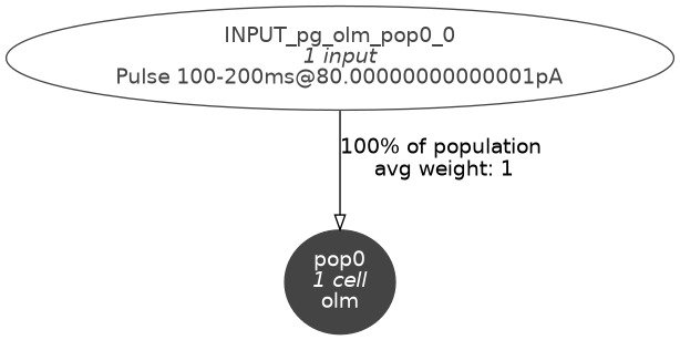
Fig. 25 Level 10 network graph generated by pynml#
Simulating the model#
Please note that this example uses the NEURON simulator to simulate the model.
Please ensure that the NEURON_HOME environment variable is correctly set as noted here.
Now that we have declared and inspected our network model and all its components, we can proceed to simulate it.
We do this in the main function:
def main():
    """Main function

    Include the NeuroML model into a LEMS simulation file, run it, plot some
    data.
    """
    # Simulation bits
    sim_id = "olm_example_sim"
    simulation = LEMSSimulation(sim_id=sim_id, duration=600, dt=0.01, simulation_seed=123)
    # Include the NeuroML model file
    simulation.include_neuroml2_file(create_olm_network())
    # Assign target for the simulation
    simulation.assign_simulation_target("single_olm_cell_network")

    # Recording information from the simulation
    simulation.create_output_file(id="output0", file_name=sim_id + ".dat")
    simulation.add_column_to_output_file("output0", column_id="pop0_0_v", quantity="pop0[0]/v")
    simulation.add_column_to_output_file("output0",
                                         column_id="pop0_0_v_Seg0_soma_0",
                                         quantity="pop0/0/olm/0/v")
    simulation.add_column_to_output_file("output0",
                                         column_id="pop0_0_v_Seg1_soma_0",
                                         quantity="pop0/0/olm/1/v")
    simulation.add_column_to_output_file("output0",
                                         column_id="pop0_0_v_Seg0_axon_0",
                                         quantity="pop0/0/olm/2/v")
    simulation.add_column_to_output_file("output0",
                                         column_id="pop0_0_v_Seg1_axon_0",
                                         quantity="pop0/0/olm/3/v")
    simulation.add_column_to_output_file("output0",
                                         column_id="pop0_0_v_Seg0_dend_0",
                                         quantity="pop0/0/olm/4/v")
    simulation.add_column_to_output_file("output0",
                                         column_id="pop0_0_v_Seg1_dend_0",
                                         quantity="pop0/0/olm/6/v")
    simulation.add_column_to_output_file("output0",
                                         column_id="pop0_0_v_Seg0_dend_1",
                                         quantity="pop0/0/olm/5/v")
    simulation.add_column_to_output_file("output0",
                                         column_id="pop0_0_v_Seg1_dend_1",
                                         quantity="pop0/0/olm/7/v")
    # Save LEMS simulation to file
    sim_file = simulation.save_to_file()

    # Run the simulation using the NEURON simulator
    pynml.run_lems_with_jneuroml_neuron(sim_file, max_memory="2G", nogui=True,
                                        plot=False, skip_run=False)
    # Plot the data
    plot_data(sim_id)
Here we first create a LEMSSimulation instance and include our network NeuroML file in it.
We must inform LEMS what the target of the simulation is.
In our case, it’s the id of our network, single_olm_cell_network:
    simulation = LEMSSimulation(sim_id=sim_id, duration=600, dt=0.01, simulation_seed=123)
    # Include the NeuroML model file
    simulation.include_neuroml2_file(create_olm_network())
    # Assign target for the simulation
    simulation.assign_simulation_target("single_olm_cell_network")
We also want to record some information, so we create an output file first with an id of output0:
simulation.add_column_to_output_file("output0", column_id="pop0_0_v", quantity="pop0[0]/v")
Now, we can record any quantity that is exposed by NeuroML (any exposure).
Here, for example, we add columns for the membrane potentials v of the different segments of the cell.
    simulation.add_column_to_output_file("output0",
                                         column_id="pop0_0_v_Seg0_soma_0",
                                         quantity="pop0/0/olm/0/v")
    simulation.add_column_to_output_file("output0",
                                         column_id="pop0_0_v_Seg1_soma_0",
                                         quantity="pop0/0/olm/1/v")
    simulation.add_column_to_output_file("output0",
                                         column_id="pop0_0_v_Seg0_axon_0",
                                         quantity="pop0/0/olm/2/v")
    simulation.add_column_to_output_file("output0",
                                         column_id="pop0_0_v_Seg1_axon_0",
                                         quantity="pop0/0/olm/3/v")
    simulation.add_column_to_output_file("output0",
                                         column_id="pop0_0_v_Seg0_dend_0",
                                         quantity="pop0/0/olm/4/v")
    simulation.add_column_to_output_file("output0",
                                         column_id="pop0_0_v_Seg1_dend_0",
                                         quantity="pop0/0/olm/6/v")
    simulation.add_column_to_output_file("output0",
                                         column_id="pop0_0_v_Seg0_dend_1",
                                         quantity="pop0/0/olm/5/v")
    simulation.add_column_to_output_file("output0",
                                         column_id="pop0_0_v_Seg1_dend_1",
                                         quantity="pop0/0/olm/7/v")
The path required to point to the quantity (exposure) to be recorded needs to be correctly provided.
Here, where we use a population list that includes an instance of the cell, it is: population_id/instance_id/cell component type/segment id/exposure. (See tickets 15 and 16)
We then save the LEMS simulation file, and run our simulation with the NEURON simulator (since the default jNeuroML simulator can only simulate single compartment cells).
    sim_file = simulation.save_to_file()

    # Run the simulation using the NEURON simulator
    pynml.run_lems_with_jneuroml_neuron(sim_file, max_memory="2G", nogui=True,
                                        plot=False, skip_run=False)
Plotting the recorded variables#
To plot the variables that we recorded, we write a simple function that reads the data and uses the generate_plot utility function which generates the membrane potential graphs for different segments.
def plot_data(sim_id):
    """Plot the sim data.

    Load the data from the file and plot the graph for the membrane potential
    using the pynml generate_plot utility function.

    :sim_id: ID of simulaton

    """
    data_array = np.loadtxt(sim_id + ".dat")
    pynml.generate_plot([data_array[:, 0]], [data_array[:, 1]], "Membrane potential (soma seg 0)", show_plot_already=False, save_figure_to=sim_id + "_seg0_soma0-v.png", xaxis="time (s)", yaxis="membrane potential (V)")
    pynml.generate_plot([data_array[:, 0]], [data_array[:, 2]], "Membrane potential (soma seg 1)", show_plot_already=False, save_figure_to=sim_id + "_seg1_soma0-v.png", xaxis="time (s)", yaxis="membrane potential (V)")
    pynml.generate_plot([data_array[:, 0]], [data_array[:, 3]], "Membrane potential (axon seg 0)", show_plot_already=False, save_figure_to=sim_id + "_seg0_axon0-v.png", xaxis="time (s)", yaxis="membrane potential (V)")
    pynml.generate_plot([data_array[:, 0]], [data_array[:, 4]], "Membrane potential (axon seg 1)", show_plot_already=False, save_figure_to=sim_id + "_seg1_axon0-v.png", xaxis="time (s)", yaxis="membrane potential (V)")
This concludes this example. Here we have seen how to create, simulate, record, and visualise a multi-compartment neuron. In the next section, you will find an interactive notebook where you can play with this example.