Optimising/fitting NeuroML Models#
pyNeuroML includes the NeuroMLTuner module for the tuning and optimisation of NeuroML models against provided data. This uses the Neurotune Python package for the fitting of models using evolutionary computation.
This page will walk through an example model optimisation.
The Python script used to run the optimisation and generate the graphs is given below. This can be adapted for other optimisations.
#!/usr/bin/env python3
"""
Example file showing the tuning of an Izhikevich neuron using pyNeuroML.

File: source/Userdocs/NML2_examples/tune-izhikevich.py

Copyright 2023 NeuroML contributors
"""


from pyneuroml.tune.NeuroMLTuner import run_optimisation
import pynwb  # type: ignore
import numpy as np
from pyelectro.utils import simple_network_analysis
from typing import List, Dict, Tuple
from pyneuroml.pynml import write_neuroml2_file
from pyneuroml.pynml import generate_plot
from pyneuroml.pynml import run_lems_with_jneuroml
from neuroml import (
    NeuroMLDocument,
    Izhikevich2007Cell,
    PulseGenerator,
    Network,
    Population,
    ExplicitInput,
)
from hdmf.container import Container
from pyneuroml.lems.LEMSSimulation import LEMSSimulation

import sys


def get_data_metrics(datafile: Container) -> Tuple[Dict, Dict, Dict]:
    """Analyse the data to get metrics to tune against.

    :returns: metrics from pyelectro analysis, currents, and the membrane potential values

    """
    analysis_results = {}
    currents = {}
    memb_vals = {}
    total_acquisitions = len(datafile.acquisition)

    for acq in range(1, total_acquisitions):
        print("Going over acquisition # {}".format(acq))

        # stimulus lasts about 1000ms, so we take about the first 1500 ms
        data_v = (
            datafile.acquisition["CurrentClampSeries_{:02d}".format(acq)].data[:15000] * 1000.0
        )
        # get sampling rate from the data
        sampling_rate = datafile.acquisition[
            "CurrentClampSeries_{:02d}".format(acq)
        ].rate
        # generate time steps from sampling rate
        data_t = np.arange(0, len(data_v) / sampling_rate, 1.0 / sampling_rate) * 1000.0
        # run the analysis
        analysis_results[acq] = simple_network_analysis({acq: data_v}, data_t)

        # extract current from description, but can be extracted from other
        # locations also, such as the CurrentClampStimulus series.
        data_i = (
            datafile.acquisition["CurrentClampSeries_{:02d}".format(acq)]
            .description.split("(")[1]
            .split("~")[1]
            .split(" ")[0]
        )
        currents[acq] = data_i
        memb_vals[acq] = (data_t, data_v)

    return (analysis_results, currents, memb_vals)


def tune_izh_model(acq_list: List, metrics_from_data: Dict, currents: Dict) -> Dict:
    """Tune networks model against the data.

    Here we generate a network with the necessary number of Izhikevich cells,
    one for each current stimulus, and tune them against the experimental data.

    :param acq_list: list of indices of acquisitions/sweeps to tune against
    :type acq_list: list
    :param metrics_from_data: dictionary with the sweep number as index, and
        the dictionary containing metrics generated from the analysis
    :type metrics_from_data: dict
    :param currents: dictionary with sweep number as index and stimulus current
        value
    """

    # length of simulation of the cells---should match the length of the
    # experiment
    sim_time = 1500.0
    # Create a NeuroML template network simulation file that we will use for
    # the tuning
    template_doc = NeuroMLDocument(id="IzhTuneNet")
    # Add an Izhikevich cell with some parameters to the document
    template_doc.izhikevich2007_cells.append(
        Izhikevich2007Cell(
            id="Izh2007",
            C="100pF",
            v0="-60mV",
            k="0.7nS_per_mV",
            vr="-60mV",
            vt="-40mV",
            vpeak="35mV",
            a="0.03per_ms",
            b="-2nS",
            c="-50.0mV",
            d="100pA",
        )
    )
    template_doc.networks.append(Network(id="Network0"))
    # Add a cell for each acquisition list
    popsize = len(acq_list)
    template_doc.networks[0].populations.append(
        Population(id="Pop0", component="Izh2007", size=popsize)
    )

    # Add a current source for each cell, matching the currents that
    # were used in the experimental study.
    counter = 0
    for acq in acq_list:
        template_doc.pulse_generators.append(
            PulseGenerator(
                id="Stim{}".format(counter),
                delay="80ms",
                duration="1000ms",
                amplitude="{}pA".format(currents[acq]),
            )
        )
        template_doc.networks[0].explicit_inputs.append(
            ExplicitInput(
                target="Pop0[{}]".format(counter), input="Stim{}".format(counter)
            )
        )
        counter = counter + 1

    # Print a summary
    print(template_doc.summary())

    # Write to a neuroml file and validate it.
    reference = "TuneIzhFergusonPyr3"
    template_filename = "{}.net.nml".format(reference)
    write_neuroml2_file(template_doc, template_filename, validate=True)

    # Now for the tuning bits

    # format is type:id/variable:id/units
    # supported types: cell/channel/izhikevich2007cell
    # supported variables:
    #  - channel: vShift
    #  - cell: channelDensity, vShift_channelDensity, channelDensityNernst,
    #  erev_id, erev_ion, specificCapacitance, resistivity
    #  - izhikevich2007Cell: all available attributes

    # we want to tune these parameters within these ranges
    # param: (min, max)
    parameters = {
        "izhikevich2007Cell:Izh2007/C/pF": (100, 300),
        "izhikevich2007Cell:Izh2007/k/nS_per_mV": (0.01, 2),
        "izhikevich2007Cell:Izh2007/vr/mV": (-70, -50),
        "izhikevich2007Cell:Izh2007/vt/mV": (-60, 0),
        "izhikevich2007Cell:Izh2007/vpeak/mV": (35, 70),
        "izhikevich2007Cell:Izh2007/a/per_ms": (0.001, 0.4),
        "izhikevich2007Cell:Izh2007/b/nS": (-10, 10),
        "izhikevich2007Cell:Izh2007/c/mV": (-65, -10),
        "izhikevich2007Cell:Izh2007/d/pA": (50, 500),
    }  # type: Dict[str, Tuple[float, float]]

    # Set up our target data and so on
    ctr = 0
    target_data = {}
    weights = {}
    for acq in acq_list:
        # data to fit to:
        # format: path/to/variable:metric
        # metric from pyelectro, for example:
        # https://pyelectro.readthedocs.io/en/latest/pyelectro.html?highlight=mean_spike_frequency#pyelectro.analysis.mean_spike_frequency
        mean_spike_frequency = "Pop0[{}]/v:mean_spike_frequency".format(ctr)
        average_last_1percent = "Pop0[{}]/v:average_last_1percent".format(ctr)
        first_spike_time = "Pop0[{}]/v:first_spike_time".format(ctr)

        # each metric can have an associated weight
        weights[mean_spike_frequency] = 1
        weights[average_last_1percent] = 1
        weights[first_spike_time] = 1

        # value of the target data from our data set
        target_data[mean_spike_frequency] = metrics_from_data[acq][
            "{}:mean_spike_frequency".format(acq)
        ]
        target_data[average_last_1percent] = metrics_from_data[acq][
            "{}:average_last_1percent".format(acq)
        ]
        target_data[first_spike_time] = metrics_from_data[acq][
            "{}:first_spike_time".format(acq)
        ]

        # only add these if the experimental data includes them
        # these are only generated for traces with spikes
        if "{}:average_maximum".format(acq) in metrics_from_data[acq]:
            average_maximum = "Pop0[{}]/v:average_maximum".format(ctr)
            weights[average_maximum] = 1
            target_data[average_maximum] = metrics_from_data[acq][
                "{}:average_maximum".format(acq)
            ]
        if "{}:average_minimum".format(acq) in metrics_from_data[acq]:
            average_minimum = "Pop0[{}]/v:average_minimum".format(ctr)
            weights[average_minimum] = 1
            target_data[average_minimum] = metrics_from_data[acq][
                "{}:average_minimum".format(acq)
            ]

        ctr = ctr + 1

    # simulator to use
    simulator = "jNeuroML"

    return run_optimisation(
        # Prefix for new files
        prefix="TuneIzh",
        # Name of the NeuroML template file
        neuroml_file=template_filename,
        # Name of the network
        target="Network0",
        # Parameters to be fitted
        parameters=list(parameters.keys()),
        # Our max and min constraints
        min_constraints=[v[0] for v in parameters.values()],
        max_constraints=[v[1] for v in parameters.values()],
        # Weights we set for parameters
        weights=weights,
        # The experimental metrics to fit to
        target_data=target_data,
        # Simulation time
        sim_time=sim_time,
        # EC parameters
        population_size=100,
        max_evaluations=500,
        num_selected=30,
        num_offspring=50,
        mutation_rate=0.9,
        num_elites=3,
        # Seed value
        seed=12345,
        # Simulator
        simulator=simulator,
        dt=0.025,
        show_plot_already='-nogui' not in sys.argv,
        save_to_file="fitted_izhikevich_fitness.png",
        save_to_file_scatter="fitted_izhikevich_scatter.png",
        save_to_file_hist="fitted_izhikevich_hist.png",
        save_to_file_output="fitted_izhikevich_output.png",
        num_parallel_evaluations=4,
    )


def run_fitted_cell_simulation(
    sweeps_to_tune_against: List, tuning_report: Dict, simulation_id: str
) -> None:
    """Run a simulation with the values obtained from the fitting

    :param tuning_report: tuning report from the optimser
    :type tuning_report: Dict
    :param simulation_id: text id of simulation
    :type simulation_id: str

    """
    # get the fittest variables
    fittest_vars = tuning_report["fittest vars"]
    C = str(fittest_vars["izhikevich2007Cell:Izh2007/C/pF"]) + "pF"
    k = str(fittest_vars["izhikevich2007Cell:Izh2007/k/nS_per_mV"]) + "nS_per_mV"
    vr = str(fittest_vars["izhikevich2007Cell:Izh2007/vr/mV"]) + "mV"
    vt = str(fittest_vars["izhikevich2007Cell:Izh2007/vt/mV"]) + "mV"
    vpeak = str(fittest_vars["izhikevich2007Cell:Izh2007/vpeak/mV"]) + "mV"
    a = str(fittest_vars["izhikevich2007Cell:Izh2007/a/per_ms"]) + "per_ms"
    b = str(fittest_vars["izhikevich2007Cell:Izh2007/b/nS"]) + "nS"
    c = str(fittest_vars["izhikevich2007Cell:Izh2007/c/mV"]) + "mV"
    d = str(fittest_vars["izhikevich2007Cell:Izh2007/d/pA"]) + "pA"

    # Create a simulation using our obtained parameters.
    # Note that the tuner generates a graph with the fitted values already, but
    # we want to keep a copy of our fitted cell also, so we'll create a NeuroML
    # Document ourselves also.
    sim_time = 1500.0
    simulation_doc = NeuroMLDocument(id="FittedNet")
    # Add an Izhikevich cell with some parameters to the document
    simulation_doc.izhikevich2007_cells.append(
        Izhikevich2007Cell(
            id="Izh2007",
            C=C,
            v0="-60mV",
            k=k,
            vr=vr,
            vt=vt,
            vpeak=vpeak,
            a=a,
            b=b,
            c=c,
            d=d,
        )
    )
    simulation_doc.networks.append(Network(id="Network0"))
    # Add a cell for each acquisition list
    popsize = len(sweeps_to_tune_against)
    simulation_doc.networks[0].populations.append(
        Population(id="Pop0", component="Izh2007", size=popsize)
    )

    # Add a current source for each cell, matching the currents that
    # were used in the experimental study.
    counter = 0
    for acq in sweeps_to_tune_against:
        simulation_doc.pulse_generators.append(
            PulseGenerator(
                id="Stim{}".format(counter),
                delay="80ms",
                duration="1000ms",
                amplitude="{}pA".format(currents[acq]),
            )
        )
        simulation_doc.networks[0].explicit_inputs.append(
            ExplicitInput(
                target="Pop0[{}]".format(counter), input="Stim{}".format(counter)
            )
        )
        counter = counter + 1

    # Print a summary
    print(simulation_doc.summary())

    # Write to a neuroml file and validate it.
    reference = "FittedIzhFergusonPyr3"
    simulation_filename = "{}.net.nml".format(reference)
    write_neuroml2_file(simulation_doc, simulation_filename, validate=True)

    simulation = LEMSSimulation(
        sim_id=simulation_id,
        duration=sim_time,
        dt=0.1,
        target="Network0",
        simulation_seed=54321,
    )
    simulation.include_neuroml2_file(simulation_filename)
    simulation.create_output_file("output0", "{}.v.dat".format(simulation_id))
    counter = 0
    for acq in sweeps_to_tune_against:
        simulation.add_column_to_output_file(
            "output0", "Pop0[{}]".format(counter), "Pop0[{}]/v".format(counter)
        )
        counter = counter + 1
    simulation_file = simulation.save_to_file()
    # simulate
    run_lems_with_jneuroml(simulation_file, max_memory="2G", nogui=True, plot=False)


def plot_sim_data(
    sweeps_to_tune_against: List, simulation_id: str, memb_pots: Dict
) -> None:
    """Plot data from our fitted simulation

    :param simulation_id: string id of simulation
    :type simulation_id: str
    """
    # Plot
    data_array = np.loadtxt("%s.v.dat" % simulation_id)

    # construct data for plotting
    counter = 0
    time_vals_list = []
    sim_v_list = []
    data_v_list = []
    data_t_list = []
    stim_vals = []
    for acq in sweeps_to_tune_against:
        stim_vals.append("{}pA".format(currents[acq]))

        # remains the same for all columns
        time_vals_list.append(data_array[:, 0] * 1000.0)
        sim_v_list.append(data_array[:, counter + 1] * 1000.0)

        data_v_list.append(memb_pots[acq][1])
        data_t_list.append(memb_pots[acq][0])

        counter = counter + 1

    # Model membrane potential plot
    generate_plot(
        xvalues=time_vals_list,
        yvalues=sim_v_list,
        labels=stim_vals,
        title="Membrane potential (model)",
        show_plot_already=False,
        save_figure_to="%s-model-v.png" % simulation_id,
        xaxis="time (ms)",
        yaxis="membrane potential (mV)",
    )
    # data membrane potential plot
    generate_plot(
        xvalues=data_t_list,
        yvalues=data_v_list,
        labels=stim_vals,
        title="Membrane potential (exp)",
        show_plot_already=False,
        save_figure_to="%s-exp-v.png" % simulation_id,
        xaxis="time (ms)",
        yaxis="membrane potential (mV)",
    )


if __name__ == "__main__":

    # set the default size for generated plots
    # https://matplotlib.org/stable/tutorials/introductory/customizing.html#a-sample-matplotlibrc-file
    import matplotlib as mpl
    mpl.rcParams["figure.figsize"] = [18, 12]

    io = pynwb.NWBHDF5IO("./FergusonEtAl2015_PYR3.nwb", "r")
    datafile = io.read()

    analysis_results, currents, memb_pots = get_data_metrics(datafile)

    # Choose what sweeps to tune against.
    # There are 33 sweeps: 1..33.
    # sweeps_to_tune_against = [1, 2, 15, 30, 31, 32, 33]
    sweeps_to_tune_against = [16,21]
    report = tune_izh_model(sweeps_to_tune_against, analysis_results, currents)

    simulation_id = "fitted_izhikevich_sim"
    run_fitted_cell_simulation(sweeps_to_tune_against, report, simulation_id)

    plot_sim_data(sweeps_to_tune_against, simulation_id, memb_pots)

    # close the data file
    io.close()
Loading data and calculating metrics to use for optimisation#
The first step in the optimisation of the model is to obtain the data that the model is to be fitted against. In this example, we will use the data set of CA1 pyramidal cell recordings using an intact whole hippocampus preparation, including recordings of rebound firing [FHA+15]. The data set is provided in the Neurodata Without Borders (NWB) format. It can can be downloaded here on the Open Source Brain repository, and can also be viewed on the NWB Explorer web application:
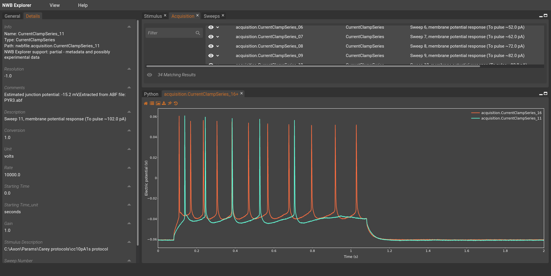
Fig. 47 Screenshot showing two recordings from FergusonEtAl2015_PYR3.nwb in NWB Explorer.#
For this example, we will use the FergusonEtAl2015_PYR3.nwb data file.
We use the PyNWB package to read it, and then pass the loaded data to our get_data_metrics function to extract the metrics we want to use for model fitting.
    io = pynwb.NWBHDF5IO("./FergusonEtAl2015_PYR3.nwb", "r")
    datafile = io.read()

    analysis_results, currents, memb_pots = get_data_metrics(datafile)
Similar to libNeuroML, PyNWB provides a Python object model to interact with NWB files. You can learn more on using PyNWB in its documentation.
Here, the data file includes recordings from multiple (33 in total) current clamp experiments that are numbered from 1 through 33.
We iterate over each recording individually to extract the membrane potential values and store them in data_v.
For each, we also calculate the time stamps for the recordings from the provided sampling rate.
We pass this information to the simple_network_analysis function provided by the PyElectro Python package to calculate features (metrics) that we will use for fitting a neuron model.
def get_data_metrics(datafile: Container) -> Tuple[Dict, Dict, Dict]:
    """Analyse the data to get metrics to tune against.

    :returns: metrics from pyelectro analysis, currents, and the membrane potential values

    """
    analysis_results = {}
    currents = {}
    memb_vals = {}
    total_acquisitions = len(datafile.acquisition)

    for acq in range(1, total_acquisitions):
        print("Going over acquisition # {}".format(acq))

        # stimulus lasts about 1000ms, so we take about the first 1500 ms
        data_v = (
            datafile.acquisition["CurrentClampSeries_{:02d}".format(acq)].data[:15000] * 1000.0
        )
        # get sampling rate from the data
        sampling_rate = datafile.acquisition[
            "CurrentClampSeries_{:02d}".format(acq)
        ].rate
        # generate time steps from sampling rate
        data_t = np.arange(0, len(data_v) / sampling_rate, 1.0 / sampling_rate) * 1000.0
        # run the analysis
        analysis_results[acq] = simple_network_analysis({acq: data_v}, data_t)

        # extract current from description, but can be extracted from other
        # locations also, such as the CurrentClampStimulus series.
        data_i = (
            datafile.acquisition["CurrentClampSeries_{:02d}".format(acq)]
            .description.split("(")[1]
            .split("~")[1]
            .split(" ")[0]
        )
        currents[acq] = data_i
        memb_vals[acq] = (data_t, data_v)

    return (analysis_results, currents, memb_vals)
The features calculated by PyElectro for each recording, which we store in analysis_results, can be seen below:
Going over acquisition # 1
pyelectro >>> {   '1:average_last_1percent': -60.4182980855306,
pyelectro >>>     '1:max_peak_no': 0,
pyelectro >>>     '1:maximum': -57.922367,
pyelectro >>>     '1:mean_spike_frequency': 0,
pyelectro >>>     '1:min_peak_no': 0,
pyelectro >>>     '1:minimum': -60.729984}
Going over acquisition # 2
pyelectro >>> {   '2:average_last_1percent': -60.2773068745931,
pyelectro >>>     '2:max_peak_no': 0,
pyelectro >>>     '2:maximum': -56.182865,
pyelectro >>>     '2:mean_spike_frequency': 0,
pyelectro >>>     '2:min_peak_no': 0,
pyelectro >>>     '2:minimum': -60.882572}
Going over acquisition # 3
pyelectro >>> {   '3:average_last_1percent': -60.175174713134766,
pyelectro >>>     '3:max_peak_no': 0,
pyelectro >>>     '3:maximum': -54.22974,
pyelectro >>>     '3:mean_spike_frequency': 0,
pyelectro >>>     '3:min_peak_no': 0,
pyelectro >>>     '3:minimum': -60.7605}
Going over acquisition # 4
pyelectro >>> {   '4:average_last_1percent': -60.11576716105143,
pyelectro >>>     '4:max_peak_no': 0,
pyelectro >>>     '4:maximum': -49.133305,
pyelectro >>>     '4:mean_spike_frequency': 0,
pyelectro >>>     '4:min_peak_no': 0,
pyelectro >>>     '4:minimum': -60.607914}
Going over acquisition # 5
pyelectro >>> {   '5:average_last_1percent': -59.628299713134766,
pyelectro >>>     '5:max_peak_no': 0,
pyelectro >>>     '5:maximum': -48.645023,
pyelectro >>>     '5:mean_spike_frequency': 0,
pyelectro >>>     '5:min_peak_no': 0,
pyelectro >>>     '5:minimum': -60.241703}
Going over acquisition # 6
pyelectro >>> {   '6:average_last_1percent': -60.04679743448893,
pyelectro >>>     '6:max_peak_no': 0,
pyelectro >>>     '6:maximum': -45.16602,
pyelectro >>>     '6:mean_spike_frequency': 0,
pyelectro >>>     '6:min_peak_no': 0,
pyelectro >>>     '6:minimum': -60.699467}
Going over acquisition # 7
pyelectro >>> {   '7:average_last_1percent': -59.88566462198893,
pyelectro >>>     '7:average_maximum': 66.3147,
pyelectro >>>     '7:average_minimum': -47.9126,
pyelectro >>>     '7:first_spike_time': 482.20000000000005,
pyelectro >>>     '7:max_peak_no': 2,
pyelectro >>>     '7:maximum': 67.38281,
pyelectro >>>     '7:mean_spike_frequency': 0,
pyelectro >>>     '7:min_peak_no': 1,
pyelectro >>>     '7:minimum': -60.15015}
Going over acquisition # 8
pyelectro >>> {   '8:average_last_1percent': -60.5531857808431,
pyelectro >>>     '8:average_maximum': 64.63623,
pyelectro >>>     '8:average_minimum': -46.05103,
pyelectro >>>     '8:first_spike_time': 280.8,
pyelectro >>>     '8:max_peak_no': 2,
pyelectro >>>     '8:maximum': 65.460205,
pyelectro >>>     '8:mean_spike_frequency': 0,
pyelectro >>>     '8:min_peak_no': 1,
pyelectro >>>     '8:minimum': -61.096195}
Going over acquisition # 9
pyelectro >>> {   '9:average_last_1percent': -60.2797482808431,
pyelectro >>>     '9:average_maximum': 62.187195,
pyelectro >>>     '9:average_minimum': -45.867924,
pyelectro >>>     '9:first_spike_time': 192.10000000000002,
pyelectro >>>     '9:interspike_time_covar': 0.12604539832023948,
pyelectro >>>     '9:max_interspike_time': 233.69999999999993,
pyelectro >>>     '9:max_peak_no': 4,
pyelectro >>>     '9:maximum': 64.42261,
pyelectro >>>     '9:mean_spike_frequency': 4.984216647283602,
pyelectro >>>     '9:min_interspike_time': 172.29999999999995,
pyelectro >>>     '9:min_peak_no': 3,
pyelectro >>>     '9:minimum': -60.91309,
pyelectro >>>     '9:peak_decay_exponent': -0.008125577959852965,
pyelectro >>>     '9:peak_linear_gradient': -0.007648055557429393,
pyelectro >>>     '9:spike_broadening': 0.891046031985908,
pyelectro >>>     '9:spike_frequency_adaptation': -0.05850411039850073,
pyelectro >>>     '9:spike_width_adaptation': 0.02767948174212246,
pyelectro >>>     '9:trough_decay_exponent': -0.00318728965696189,
pyelectro >>>     '9:trough_phase_adaptation': -0.05016262394149966}
Going over acquisition # 10
pyelectro >>> {   '10:average_last_1percent': -60.4292844136556,
pyelectro >>>     '10:average_maximum': 59.680183,
pyelectro >>>     '10:average_minimum': -44.731144,
pyelectro >>>     '10:first_spike_time': 156.9,
pyelectro >>>     '10:interspike_time_covar': 0.5779639183148945,
pyelectro >>>     '10:max_interspike_time': 438.5000000000001,
pyelectro >>>     '10:max_peak_no': 5,
pyelectro >>>     '10:maximum': 62.072758,
pyelectro >>>     '10:mean_spike_frequency': 4.553215708594194,
pyelectro >>>     '10:min_interspike_time': 132.60000000000005,
pyelectro >>>     '10:min_peak_no': 4,
pyelectro >>>     '10:minimum': -60.882572,
pyelectro >>>     '10:peak_decay_exponent': -0.009585017031582235,
pyelectro >>>     '10:peak_linear_gradient': -0.005260966229876463,
pyelectro >>>     '10:spike_broadening': 0.8756680523402136,
pyelectro >>>     '10:spike_frequency_adaptation': -0.04780471479504103,
pyelectro >>>     '10:spike_width_adaptation': 0.014551159295128686,
pyelectro >>>     '10:trough_decay_exponent': -0.006056437839814275,
pyelectro >>>     '10:trough_phase_adaptation': -0.04269124477477909}
Going over acquisition # 11
pyelectro >>> {   '11:average_last_1percent': -60.84635798136393,
pyelectro >>>     '11:average_maximum': 58.73414,
pyelectro >>>     '11:average_minimum': -43.800358,
pyelectro >>>     '11:first_spike_time': 138.1,
pyelectro >>>     '11:interspike_time_covar': 0.18317620745649893,
pyelectro >>>     '11:max_interspike_time': 179.9999999999999,
pyelectro >>>     '11:max_peak_no': 5,
pyelectro >>>     '11:maximum': 61.03516,
pyelectro >>>     '11:mean_spike_frequency': 7.033585370142431,
pyelectro >>>     '11:min_interspike_time': 106.50000000000003,
pyelectro >>>     '11:min_peak_no': 4,
pyelectro >>>     '11:minimum': -61.248783,
pyelectro >>>     '11:peak_decay_exponent': -0.010372120562797708,
pyelectro >>>     '11:peak_linear_gradient': -0.0074866848970347325,
pyelectro >>>     '11:spike_broadening': 0.8498887121142943,
pyelectro >>>     '11:spike_frequency_adaptation': -0.052381521145715274,
pyelectro >>>     '11:spike_width_adaptation': 0.025414793671653328,
pyelectro >>>     '11:trough_decay_exponent': -0.007552906636393599,
pyelectro >>>     '11:trough_phase_adaptation': -0.04473631982885844}
Going over acquisition # 12
pyelectro >>> {   '12:average_last_1percent': -61.085208892822266,
pyelectro >>>     '12:average_maximum': 58.481857,
pyelectro >>>     '12:average_minimum': -42.974857,
pyelectro >>>     '12:first_spike_time': 127.40000000000002,
pyelectro >>>     '12:interspike_time_covar': 0.16275057704467177,
pyelectro >>>     '12:max_interspike_time': 136.5,
pyelectro >>>     '12:max_peak_no': 6,
pyelectro >>>     '12:maximum': 61.737064,
pyelectro >>>     '12:mean_spike_frequency': 8.791981712678037,
pyelectro >>>     '12:min_interspike_time': 84.60000000000001,
pyelectro >>>     '12:min_peak_no': 5,
pyelectro >>>     '12:minimum': -61.462406,
pyelectro >>>     '12:peak_decay_exponent': -0.015987075984851808,
pyelectro >>>     '12:peak_linear_gradient': -0.009383652380440125,
pyelectro >>>     '12:spike_broadening': 0.8205694396572242,
pyelectro >>>     '12:spike_frequency_adaptation': -0.04259621402895674,
pyelectro >>>     '12:spike_width_adaptation': 0.0228428573204052,
pyelectro >>>     '12:trough_decay_exponent': -0.012180031782655684,
pyelectro >>>     '12:trough_phase_adaptation': 0.0003391093549627843}
Going over acquisition # 13
pyelectro >>> {   '13:average_last_1percent': -60.6233762105306,
pyelectro >>>     '13:average_maximum': 56.980137,
pyelectro >>>     '13:average_minimum': -42.205814,
pyelectro >>>     '13:first_spike_time': 122.9,
pyelectro >>>     '13:interspike_time_covar': 0.1989630987796946,
pyelectro >>>     '13:max_interspike_time': 138.9000000000001,
pyelectro >>>     '13:max_peak_no': 8,
pyelectro >>>     '13:maximum': 61.30982,
pyelectro >>>     '13:mean_spike_frequency': 9.743875278396434,
pyelectro >>>     '13:min_interspike_time': 75.4,
pyelectro >>>     '13:min_peak_no': 7,
pyelectro >>>     '13:minimum': -60.974125,
pyelectro >>>     '13:peak_decay_exponent': -0.01856642711769415,
pyelectro >>>     '13:peak_linear_gradient': -0.009561076077386068,
pyelectro >>>     '13:spike_broadening': 0.803052014150605,
pyelectro >>>     '13:spike_frequency_adaptation': -0.028079821139188187,
pyelectro >>>     '13:spike_width_adaptation': 0.01504310702538977,
pyelectro >>>     '13:trough_decay_exponent': -0.013208504624154408,
pyelectro >>>     '13:trough_phase_adaptation': -0.025379665674913895}
Going over acquisition # 14
pyelectro >>> {   '14:average_last_1percent': -60.723270416259766,
pyelectro >>>     '14:average_maximum': 55.986195,
pyelectro >>>     '14:average_minimum': -41.54587,
pyelectro >>>     '14:first_spike_time': 114.8,
pyelectro >>>     '14:interspike_time_covar': 0.34335772265161896,
pyelectro >>>     '14:max_interspike_time': 194.39999999999998,
pyelectro >>>     '14:max_peak_no': 9,
pyelectro >>>     '14:maximum': 60.882572,
pyelectro >>>     '14:mean_spike_frequency': 8.785416209092906,
pyelectro >>>     '14:min_interspike_time': 74.40000000000002,
pyelectro >>>     '14:min_peak_no': 8,
pyelectro >>>     '14:minimum': -61.126713,
pyelectro >>>     '14:peak_decay_exponent': -0.022541304298167242,
pyelectro >>>     '14:peak_linear_gradient': -0.008000988888256885,
pyelectro >>>     '14:spike_broadening': 0.8009562042583951,
pyelectro >>>     '14:spike_frequency_adaptation': -0.022434594832088855,
pyelectro >>>     '14:spike_width_adaptation': 0.010424354074822617,
pyelectro >>>     '14:trough_decay_exponent': -0.018754566142487872,
pyelectro >>>     '14:trough_phase_adaptation': -0.019014319738344054}
Going over acquisition # 15
pyelectro >>> {   '15:average_last_1percent': -60.99833552042643,
pyelectro >>>     '15:average_maximum': 55.89295,
pyelectro >>>     '15:average_minimum': -40.78892,
pyelectro >>>     '15:first_spike_time': 113.2,
pyelectro >>>     '15:interspike_time_covar': 0.6436697297327385,
pyelectro >>>     '15:max_interspike_time': 311.30000000000007,
pyelectro >>>     '15:max_peak_no': 8,
pyelectro >>>     '15:maximum': 60.91309,
pyelectro >>>     '15:mean_spike_frequency': 8.201523140011716,
pyelectro >>>     '15:min_interspike_time': 71.60000000000001,
pyelectro >>>     '15:min_peak_no': 7,
pyelectro >>>     '15:minimum': -61.370853,
pyelectro >>>     '15:peak_decay_exponent': -0.025953113905923406,
pyelectro >>>     '15:peak_linear_gradient': -0.008306657481016694,
pyelectro >>>     '15:spike_broadening': 0.7782197474305453,
pyelectro >>>     '15:spike_frequency_adaptation': -0.030010388928284993,
pyelectro >>>     '15:spike_width_adaptation': 0.012108100430332605,
pyelectro >>>     '15:trough_decay_exponent': -0.01262141611091244,
pyelectro >>>     '15:trough_phase_adaptation': -0.025746376793896804}
Going over acquisition # 16
pyelectro >>> {   '16:average_last_1percent': -60.380863189697266,
pyelectro >>>     '16:average_maximum': 54.52382,
pyelectro >>>     '16:average_minimum': -39.78882,
pyelectro >>>     '16:first_spike_time': 108.9,
pyelectro >>>     '16:interspike_time_covar': 0.23652534644271225,
pyelectro >>>     '16:max_interspike_time': 123.00000000000011,
pyelectro >>>     '16:max_peak_no': 11,
pyelectro >>>     '16:maximum': 60.7605,
pyelectro >>>     '16:mean_spike_frequency': 10.8837614279495,
pyelectro >>>     '16:min_interspike_time': 59.30000000000001,
pyelectro >>>     '16:min_peak_no': 10,
pyelectro >>>     '16:minimum': -60.79102,
pyelectro >>>     '16:peak_decay_exponent': -0.03301104578192642,
pyelectro >>>     '16:peak_linear_gradient': -0.007545664792227554,
pyelectro >>>     '16:spike_broadening': 0.7546314677569799,
pyelectro >>>     '16:spike_frequency_adaptation': -0.013692136410690963,
pyelectro >>>     '16:spike_width_adaptation': 0.008664177864358623,
pyelectro >>>     '16:trough_decay_exponent': -0.023836469122601508,
pyelectro >>>     '16:trough_phase_adaptation': -0.010081239597430595}
Going over acquisition # 17
pyelectro >>> {   '17:average_last_1percent': -60.552982330322266,
pyelectro >>>     '17:average_maximum': 54.44642,
pyelectro >>>     '17:average_minimum': -39.008247,
pyelectro >>>     '17:first_spike_time': 105.6,
pyelectro >>>     '17:interspike_time_covar': 0.19651182311074483,
pyelectro >>>     '17:max_interspike_time': 106.29999999999995,
pyelectro >>>     '17:max_peak_no': 10,
pyelectro >>>     '17:maximum': 60.63843,
pyelectro >>>     '17:mean_spike_frequency': 11.506008693428791,
pyelectro >>>     '17:min_interspike_time': 58.60000000000002,
pyelectro >>>     '17:min_peak_no': 9,
pyelectro >>>     '17:minimum': -61.03516,
pyelectro >>>     '17:peak_decay_exponent': -0.03684157763477531,
pyelectro >>>     '17:peak_linear_gradient': -0.009090863209461205,
pyelectro >>>     '17:spike_broadening': 0.7534694949245309,
pyelectro >>>     '17:spike_frequency_adaptation': -0.023373852901912264,
pyelectro >>>     '17:spike_width_adaptation': 0.011268432654001511,
pyelectro >>>     '17:trough_decay_exponent': -0.020590018720385343,
pyelectro >>>     '17:trough_phase_adaptation': -0.00906121257722172}
Going over acquisition # 18
pyelectro >>> {   '18:average_last_1percent': -60.64799372355143,
pyelectro >>>     '18:average_maximum': 53.783077,
pyelectro >>>     '18:average_minimum': -38.424683,
pyelectro >>>     '18:first_spike_time': 104.2,
pyelectro >>>     '18:interspike_time_covar': 0.2502832189694502,
pyelectro >>>     '18:max_interspike_time': 124.59999999999991,
pyelectro >>>     '18:max_peak_no': 11,
pyelectro >>>     '18:maximum': 60.63843,
pyelectro >>>     '18:mean_spike_frequency': 11.420740063956146,
pyelectro >>>     '18:min_interspike_time': 53.09999999999998,
pyelectro >>>     '18:min_peak_no': 10,
pyelectro >>>     '18:minimum': -61.03516,
pyelectro >>>     '18:peak_decay_exponent': -0.04141134556729957,
pyelectro >>>     '18:peak_linear_gradient': -0.008476351143979814,
pyelectro >>>     '18:spike_broadening': 0.7403041191114148,
pyelectro >>>     '18:spike_frequency_adaptation': -0.01809717600857398,
pyelectro >>>     '18:spike_width_adaptation': 0.009174879706803092,
pyelectro >>>     '18:trough_decay_exponent': -0.02760451378209885,
pyelectro >>>     '18:trough_phase_adaptation': -0.005774543184281237}
Going over acquisition # 19
pyelectro >>> {   '19:average_last_1percent': -60.855106353759766,
pyelectro >>>     '19:average_maximum': 53.430737,
pyelectro >>>     '19:average_minimum': -37.713623,
pyelectro >>>     '19:first_spike_time': 102.50000000000001,
pyelectro >>>     '19:interspike_time_covar': 0.25333327224227414,
pyelectro >>>     '19:max_interspike_time': 114.69999999999993,
pyelectro >>>     '19:max_peak_no': 11,
pyelectro >>>     '19:maximum': 60.607914,
pyelectro >>>     '19:mean_spike_frequency': 12.47038284075321,
pyelectro >>>     '19:min_interspike_time': 51.8,
pyelectro >>>     '19:min_peak_no': 10,
pyelectro >>>     '19:minimum': -61.248783,
pyelectro >>>     '19:peak_decay_exponent': -0.04918301935790627,
pyelectro >>>     '19:peak_linear_gradient': -0.008553290998046907,
pyelectro >>>     '19:spike_broadening': 0.7301692622822238,
pyelectro >>>     '19:spike_frequency_adaptation': -0.015561797159916213,
pyelectro >>>     '19:spike_width_adaptation': 0.010054185105794627,
pyelectro >>>     '19:trough_decay_exponent': -0.03413795061471875,
pyelectro >>>     '19:trough_phase_adaptation': -0.011967671377256838}
Going over acquisition # 20
pyelectro >>> {   '20:average_last_1percent': -60.793460845947266,
pyelectro >>>     '20:average_maximum': 53.11169,
pyelectro >>>     '20:average_minimum': -37.045288,
pyelectro >>>     '20:first_spike_time': 101.4,
pyelectro >>>     '20:interspike_time_covar': 0.2865607615520669,
pyelectro >>>     '20:max_interspike_time': 123.0,
pyelectro >>>     '20:max_peak_no': 11,
pyelectro >>>     '20:maximum': 60.51636,
pyelectro >>>     '20:mean_spike_frequency': 12.624668602449184,
pyelectro >>>     '20:min_interspike_time': 49.099999999999994,
pyelectro >>>     '20:min_peak_no': 10,
pyelectro >>>     '20:minimum': -61.30982,
pyelectro >>>     '20:peak_decay_exponent': -0.053836942989781186,
pyelectro >>>     '20:peak_linear_gradient': -0.009554089132365705,
pyelectro >>>     '20:spike_broadening': 0.7067401817806985,
pyelectro >>>     '20:spike_frequency_adaptation': -0.02046601020346991,
pyelectro >>>     '20:spike_width_adaptation': 0.01032699280307952,
pyelectro >>>     '20:trough_decay_exponent': -0.03229413870032492,
pyelectro >>>     '20:trough_phase_adaptation': -0.009902402143729637}
Going over acquisition # 21
pyelectro >>> {   '21:average_last_1percent': -59.912113189697266,
pyelectro >>>     '21:average_maximum': 51.912754,
pyelectro >>>     '21:average_minimum': -35.964966,
pyelectro >>>     '21:first_spike_time': 100.4,
pyelectro >>>     '21:interspike_time_covar': 0.31784939578511834,
pyelectro >>>     '21:max_interspike_time': 130.10000000000002,
pyelectro >>>     '21:max_peak_no': 13,
pyelectro >>>     '21:maximum': 61.15723,
pyelectro >>>     '21:mean_spike_frequency': 12.369858777445623,
pyelectro >>>     '21:min_interspike_time': 45.10000000000002,
pyelectro >>>     '21:min_peak_no': 12,
pyelectro >>>     '21:minimum': -61.614994,
pyelectro >>>     '21:peak_decay_exponent': -0.06340663337165775,
pyelectro >>>     '21:peak_linear_gradient': -0.009514554022982258,
pyelectro >>>     '21:spike_broadening': 0.6805457955255507,
pyelectro >>>     '21:spike_frequency_adaptation': -0.012321447021551269,
pyelectro >>>     '21:spike_width_adaptation': 0.007303096579113352,
pyelectro >>>     '21:trough_decay_exponent': -0.03236374133246423,
pyelectro >>>     '21:trough_phase_adaptation': -0.009705621425080494}
Going over acquisition # 22
pyelectro >>> {   '22:average_last_1percent': -60.0850461324056,
pyelectro >>>     '22:average_maximum': 51.325874,
pyelectro >>>     '22:average_minimum': -35.22746,
pyelectro >>>     '22:first_spike_time': 97.7,
pyelectro >>>     '22:interspike_time_covar': 0.3280130255436152,
pyelectro >>>     '22:max_interspike_time': 123.30000000000007,
pyelectro >>>     '22:max_peak_no': 13,
pyelectro >>>     '22:maximum': 60.91309,
pyelectro >>>     '22:mean_spike_frequency': 12.784998934583422,
pyelectro >>>     '22:min_interspike_time': 40.60000000000001,
pyelectro >>>     '22:min_peak_no': 12,
pyelectro >>>     '22:minimum': -60.51636,
pyelectro >>>     '22:peak_decay_exponent': -0.07398649685748288,
pyelectro >>>     '22:peak_linear_gradient': -0.008846573199048182,
pyelectro >>>     '22:spike_broadening': 0.673572178798493,
pyelectro >>>     '22:spike_frequency_adaptation': -0.01394751742502263,
pyelectro >>>     '22:spike_width_adaptation': 0.00745978471908774,
pyelectro >>>     '22:trough_decay_exponent': -0.03985576781966312,
pyelectro >>>     '22:trough_phase_adaptation': -0.012949190338366346}
Going over acquisition # 23
pyelectro >>> {   '23:average_last_1percent': -60.42582575480143,
pyelectro >>>     '23:average_maximum': 50.883705,
pyelectro >>>     '23:average_minimum': -34.70553,
pyelectro >>>     '23:first_spike_time': 97.0,
pyelectro >>>     '23:interspike_time_covar': 0.3025008293643565,
pyelectro >>>     '23:max_interspike_time': 113.00000000000011,
pyelectro >>>     '23:max_peak_no': 14,
pyelectro >>>     '23:maximum': 61.126713,
pyelectro >>>     '23:mean_spike_frequency': 13.453378867846421,
pyelectro >>>     '23:min_interspike_time': 37.599999999999994,
pyelectro >>>     '23:min_peak_no': 13,
pyelectro >>>     '23:minimum': -60.79102,
pyelectro >>>     '23:peak_decay_exponent': -0.09454776279913378,
pyelectro >>>     '23:peak_linear_gradient': -0.007913299554316041,
pyelectro >>>     '23:spike_broadening': 0.6664213397577756,
pyelectro >>>     '23:spike_frequency_adaptation': -0.014974747741974222,
pyelectro >>>     '23:spike_width_adaptation': 0.0067844847504214744,
pyelectro >>>     '23:trough_decay_exponent': -0.04357925225307838,
pyelectro >>>     '23:trough_phase_adaptation': -0.006437508651280852}
Going over acquisition # 24
pyelectro >>> {   '24:average_last_1percent': -60.48380915323893,
pyelectro >>>     '24:average_maximum': 50.66572,
pyelectro >>>     '24:average_minimum': -34.043533,
pyelectro >>>     '24:first_spike_time': 95.9,
pyelectro >>>     '24:interspike_time_covar': 0.2757061784222999,
pyelectro >>>     '24:max_interspike_time': 106.29999999999995,
pyelectro >>>     '24:max_peak_no': 14,
pyelectro >>>     '24:maximum': 61.2793,
pyelectro >>>     '24:mean_spike_frequency': 13.685651121170649,
pyelectro >>>     '24:min_interspike_time': 42.5,
pyelectro >>>     '24:min_peak_no': 13,
pyelectro >>>     '24:minimum': -61.03516,
pyelectro >>>     '24:peak_decay_exponent': -0.10291055243646331,
pyelectro >>>     '24:peak_linear_gradient': -0.008156801002617309,
pyelectro >>>     '24:spike_broadening': 0.647962840377368,
pyelectro >>>     '24:spike_frequency_adaptation': -0.01033640102347251,
pyelectro >>>     '24:spike_width_adaptation': 0.0070544336550024695,
pyelectro >>>     '24:trough_decay_exponent': -0.04136814132208841,
pyelectro >>>     '24:trough_phase_adaptation': -0.007165702258804302}
Going over acquisition # 25
pyelectro >>> {   '25:average_last_1percent': -60.056766510009766,
pyelectro >>>     '25:average_maximum': 50.34093,
pyelectro >>>     '25:average_minimum': -33.228947,
pyelectro >>>     '25:first_spike_time': 95.60000000000001,
pyelectro >>>     '25:interspike_time_covar': 0.28833246313094774,
pyelectro >>>     '25:max_interspike_time': 100.80000000000007,
pyelectro >>>     '25:max_peak_no': 14,
pyelectro >>>     '25:maximum': 61.40137,
pyelectro >>>     '25:mean_spike_frequency': 14.023732470334416,
pyelectro >>>     '25:min_interspike_time': 39.10000000000001,
pyelectro >>>     '25:min_peak_no': 13,
pyelectro >>>     '25:minimum': -60.607914,
pyelectro >>>     '25:peak_decay_exponent': -0.1047695739806843,
pyelectro >>>     '25:peak_linear_gradient': -0.00879119329941481,
pyelectro >>>     '25:spike_broadening': 0.6394636967007732,
pyelectro >>>     '25:spike_frequency_adaptation': -0.011357738090467376,
pyelectro >>>     '25:spike_width_adaptation': 0.007198805900434394,
pyelectro >>>     '25:trough_decay_exponent': -0.03898706127522965,
pyelectro >>>     '25:trough_phase_adaptation': -0.005791081007349543}
Going over acquisition # 26
pyelectro >>> {   '26:average_last_1percent': -60.2272580464681,
pyelectro >>>     '26:average_maximum': 49.776356,
pyelectro >>>     '26:average_minimum': -32.534084,
pyelectro >>>     '26:first_spike_time': 94.89999999999999,
pyelectro >>>     '26:interspike_time_covar': 0.3174070553930572,
pyelectro >>>     '26:max_interspike_time': 115.70000000000005,
pyelectro >>>     '26:max_peak_no': 14,
pyelectro >>>     '26:maximum': 61.15723,
pyelectro >>>     '26:mean_spike_frequency': 14.697569248162802,
pyelectro >>>     '26:min_interspike_time': 35.60000000000001,
pyelectro >>>     '26:min_peak_no': 13,
pyelectro >>>     '26:minimum': -60.729984,
pyelectro >>>     '26:peak_decay_exponent': -0.11931629839276492,
pyelectro >>>     '26:peak_linear_gradient': -0.009603020729143796,
pyelectro >>>     '26:spike_broadening': 0.6253471365146865,
pyelectro >>>     '26:spike_frequency_adaptation': -0.015585439927950483,
pyelectro >>>     '26:spike_width_adaptation': 0.007759081127414656,
pyelectro >>>     '26:trough_decay_exponent': -0.049101688628808246,
pyelectro >>>     '26:trough_phase_adaptation': -0.012139424609633551}
Going over acquisition # 27
pyelectro >>> {   '27:average_last_1percent': -60.3578732808431,
pyelectro >>>     '27:average_maximum': 49.30769,
pyelectro >>>     '27:average_minimum': -32.003548,
pyelectro >>>     '27:first_spike_time': 93.60000000000001,
pyelectro >>>     '27:interspike_time_covar': 0.309017296765978,
pyelectro >>>     '27:max_interspike_time': 109.0,
pyelectro >>>     '27:max_peak_no': 14,
pyelectro >>>     '27:maximum': 61.43189,
pyelectro >>>     '27:mean_spike_frequency': 14.729209154769997,
pyelectro >>>     '27:min_interspike_time': 32.19999999999999,
pyelectro >>>     '27:min_peak_no': 13,
pyelectro >>>     '27:minimum': -60.7605,
pyelectro >>>     '27:peak_decay_exponent': -0.12538878925370048,
pyelectro >>>     '27:peak_linear_gradient': -0.009067695791685005,
pyelectro >>>     '27:spike_broadening': 0.6066765033439258,
pyelectro >>>     '27:spike_frequency_adaptation': -0.015492078035720953,
pyelectro >>>     '27:spike_width_adaptation': 0.007539073044770246,
pyelectro >>>     '27:trough_decay_exponent': -0.05115040330367209,
pyelectro >>>     '27:trough_phase_adaptation': -0.012545852013557039}
Going over acquisition # 28
pyelectro >>> {   '28:average_last_1percent': -60.3798459370931,
pyelectro >>>     '28:average_maximum': 48.999027,
pyelectro >>>     '28:average_minimum': -31.055996,
pyelectro >>>     '28:first_spike_time': 93.4,
pyelectro >>>     '28:interspike_time_covar': 0.30636145843159784,
pyelectro >>>     '28:max_interspike_time': 104.70000000000005,
pyelectro >>>     '28:max_peak_no': 15,
pyelectro >>>     '28:maximum': 61.2793,
pyelectro >>>     '28:mean_spike_frequency': 14.760147601476012,
pyelectro >>>     '28:min_interspike_time': 34.20000000000002,
pyelectro >>>     '28:min_peak_no': 14,
pyelectro >>>     '28:minimum': -60.943607,
pyelectro >>>     '28:peak_decay_exponent': -0.16496940386452533,
pyelectro >>>     '28:peak_linear_gradient': -0.007631694348641044,
pyelectro >>>     '28:spike_broadening': 0.5953810644123492,
pyelectro >>>     '28:spike_frequency_adaptation': -0.014342884276047468,
pyelectro >>>     '28:spike_width_adaptation': 0.006650416835633624,
pyelectro >>>     '28:trough_decay_exponent': -0.04668774074305247,
pyelectro >>>     '28:trough_phase_adaptation': 0.006738292518776989}
Going over acquisition # 29
pyelectro >>> {   '29:average_last_1percent': -60.662235260009766,
pyelectro >>>     '29:average_maximum': 48.664642,
pyelectro >>>     '29:average_minimum': -30.39551,
pyelectro >>>     '29:first_spike_time': 93.10000000000001,
pyelectro >>>     '29:interspike_time_covar': 0.5343365146969321,
pyelectro >>>     '29:max_interspike_time': 183.60000000000002,
pyelectro >>>     '29:max_peak_no': 14,
pyelectro >>>     '29:maximum': 61.370853,
pyelectro >>>     '29:mean_spike_frequency': 14.458903347792235,
pyelectro >>>     '29:min_interspike_time': 25.599999999999994,
pyelectro >>>     '29:min_peak_no': 13,
pyelectro >>>     '29:minimum': -61.187748,
pyelectro >>>     '29:peak_decay_exponent': -0.15153571047754788,
pyelectro >>>     '29:peak_linear_gradient': -0.007862338819211844,
pyelectro >>>     '29:spike_broadening': 0.5870269764023183,
pyelectro >>>     '29:spike_frequency_adaptation': -0.016055090374903703,
pyelectro >>>     '29:spike_width_adaptation': 0.00754720476623759,
pyelectro >>>     '29:trough_decay_exponent': -0.05167436400749407,
pyelectro >>>     '29:trough_phase_adaptation': 0.006928896725677521}
Going over acquisition # 30
pyelectro >>> {   '30:average_last_1percent': -60.68766657511393,
pyelectro >>>     '30:average_maximum': 48.13843,
pyelectro >>>     '30:average_minimum': -29.626032,
pyelectro >>>     '30:first_spike_time': 92.80000000000001,
pyelectro >>>     '30:interspike_time_covar': 0.34247923269889735,
pyelectro >>>     '30:max_interspike_time': 103.89999999999998,
pyelectro >>>     '30:max_peak_no': 15,
pyelectro >>>     '30:maximum': 61.767582,
pyelectro >>>     '30:mean_spike_frequency': 15.688032272523532,
pyelectro >>>     '30:min_interspike_time': 24.599999999999994,
pyelectro >>>     '30:min_peak_no': 14,
pyelectro >>>     '30:minimum': -61.248783,
pyelectro >>>     '30:peak_decay_exponent': -0.19194537406993217,
pyelectro >>>     '30:peak_linear_gradient': -0.006994401512067068,
pyelectro >>>     '30:spike_broadening': 0.5770492253613585,
pyelectro >>>     '30:spike_frequency_adaptation': -0.01538364588730742,
pyelectro >>>     '30:spike_width_adaptation': 0.0069293286774622966,
pyelectro >>>     '30:trough_decay_exponent': -0.04326627973106321,
pyelectro >>>     '30:trough_phase_adaptation': 0.0064812799362231775}
Going over acquisition # 31
pyelectro >>> {   '31:average_last_1percent': -60.63212458292643,
pyelectro >>>     '31:average_maximum': 48.024498,
pyelectro >>>     '31:average_minimum': -29.024399,
pyelectro >>>     '31:first_spike_time': 92.4,
pyelectro >>>     '31:interspike_time_covar': 0.406847478416553,
pyelectro >>>     '31:max_interspike_time': 133.5999999999999,
pyelectro >>>     '31:max_peak_no': 15,
pyelectro >>>     '31:maximum': 61.889652,
pyelectro >>>     '31:mean_spike_frequency': 14.704337779644996,
pyelectro >>>     '31:min_interspike_time': 29.5,
pyelectro >>>     '31:min_peak_no': 14,
pyelectro >>>     '31:minimum': -61.30982,
pyelectro >>>     '31:peak_decay_exponent': -0.1671016453568311,
pyelectro >>>     '31:peak_linear_gradient': -0.0086990196695813,
pyelectro >>>     '31:spike_broadening': 0.5569432887124698,
pyelectro >>>     '31:spike_frequency_adaptation': -0.014767300558908368,
pyelectro >>>     '31:spike_width_adaptation': 0.006743383637276833,
pyelectro >>>     '31:trough_decay_exponent': -0.04051025499900451,
pyelectro >>>     '31:trough_phase_adaptation': 0.006526251236739548}
Going over acquisition # 32
pyelectro >>> {   '32:average_last_1percent': -59.76054255167643,
pyelectro >>>     '32:average_maximum': 47.896324,
pyelectro >>>     '32:average_minimum': -27.88653,
pyelectro >>>     '32:first_spike_time': 91.30000000000001,
pyelectro >>>     '32:interspike_time_covar': 0.34354448310799324,
pyelectro >>>     '32:max_interspike_time': 106.60000000000002,
pyelectro >>>     '32:max_peak_no': 15,
pyelectro >>>     '32:maximum': 62.469486,
pyelectro >>>     '32:mean_spike_frequency': 15.222355115798628,
pyelectro >>>     '32:min_interspike_time': 30.700000000000003,
pyelectro >>>     '32:min_peak_no': 14,
pyelectro >>>     '32:minimum': -60.42481,
pyelectro >>>     '32:peak_decay_exponent': -0.2052962133940038,
pyelectro >>>     '32:peak_linear_gradient': -0.00818069814788547,
pyelectro >>>     '32:spike_broadening': 0.5505132639070699,
pyelectro >>>     '32:spike_frequency_adaptation': -0.0127147931736426,
pyelectro >>>     '32:spike_width_adaptation': 0.006794945084249822,
pyelectro >>>     '32:trough_decay_exponent': -0.045165955567810896,
pyelectro >>>     '32:trough_phase_adaptation': 0.00648520248429949}
Going over acquisition # 33
pyelectro >>> {   '33:average_last_1percent': -59.76237360636393,
pyelectro >>>     '33:average_maximum': 47.544212,
pyelectro >>>     '33:average_minimum': -27.22403,
pyelectro >>>     '33:first_spike_time': 91.4,
pyelectro >>>     '33:interspike_time_covar': 0.9530683477414146,
pyelectro >>>     '33:max_interspike_time': 322.6,
pyelectro >>>     '33:max_peak_no': 14,
pyelectro >>>     '33:maximum': 62.28638,
pyelectro >>>     '33:mean_spike_frequency': 13.151239251390995,
pyelectro >>>     '33:min_interspike_time': 29.0,
pyelectro >>>     '33:min_peak_no': 13,
pyelectro >>>     '33:minimum': -60.42481,
pyelectro >>>     '33:peak_decay_exponent': -0.21944646857580366,
pyelectro >>>     '33:peak_linear_gradient': -0.00986060329457358,
pyelectro >>>     '33:spike_broadening': 0.5524597059029492,
pyelectro >>>     '33:spike_frequency_adaptation': -0.01666625273183203,
pyelectro >>>     '33:spike_width_adaptation': 0.006743589954469429,
pyelectro >>>     '33:trough_decay_exponent': -0.03685620725832345,
pyelectro >>>     '33:trough_phase_adaptation': -0.012225503917922204}
We now have the following information:
analysis_results: the results of the analysis by PyElectro; we need these to set the target values for our fittingcurrents: the value of stimulation current for each sweep we’ve chosen; we need this for our modelsmemb_vals: the time series of the membrane potentials and recordings times; we’ll use this to plot the membrane potentials later to compare our fitted model against
Running the optimisation#
To run the optimisation, we want to choose which of the 33 time series we want to fit our model against. Ideally, we would want to fit our model to all of them. Here, however, for simplicity and to keep the computation time in check, we only pick two of the 33 sweeps. (As an exercise, you can change the list to see how that affects your fitting.)
    sweeps_to_tune_against = [16,21]
    report = tune_izh_model(sweeps_to_tune_against, analysis_results, currents)
The Neurotune optimiser uses the evolutionary computation method provided by the Inspyred package. In short:
the evolutionary algorithm starts with a population of models, each with a random value for a set of parameters constrained by a max/min value we have supplied
it then calculates a fitness value for each model by comparing the features generated by the model to the target features that we provide
in each generation, it finds the fittest models (parents)
it mutates these to generate the next generation of models (offspring)
it replaces the least fit models with fittest of the new individuals
The idea is that by calculating the fittest parents and offspring, it will find the candidate models that fit the provided target data best. You can read more about evolutionary computation online (e.g. Wikipedia). More information on model fitting in computational neuroscience can also be found in the literature. For example, see this review [PBM04, RGF+11].
Here, we follow the following steps:
we set up a template NeuroML model that will be passed to the optimiser
we list the parameters we want to fit, and provide the extents of their state spaces
we list the target features that the optimiser will use to calculate fitness, and set their weights
finally, we use the
run_optimisationfunction to run the optimisation
The tune_izh_model function shown below is the main workhorse function that does our fitting:
def tune_izh_model(acq_list: List, metrics_from_data: Dict, currents: Dict) -> Dict:
    """Tune networks model against the data.

    Here we generate a network with the necessary number of Izhikevich cells,
    one for each current stimulus, and tune them against the experimental data.

    :param acq_list: list of indices of acquisitions/sweeps to tune against
    :type acq_list: list
    :param metrics_from_data: dictionary with the sweep number as index, and
        the dictionary containing metrics generated from the analysis
    :type metrics_from_data: dict
    :param currents: dictionary with sweep number as index and stimulus current
        value
    """

    # length of simulation of the cells---should match the length of the
    # experiment
    sim_time = 1500.0
    # Create a NeuroML template network simulation file that we will use for
    # the tuning
    template_doc = NeuroMLDocument(id="IzhTuneNet")
    # Add an Izhikevich cell with some parameters to the document
    template_doc.izhikevich2007_cells.append(
        Izhikevich2007Cell(
            id="Izh2007",
            C="100pF",
            v0="-60mV",
            k="0.7nS_per_mV",
            vr="-60mV",
            vt="-40mV",
            vpeak="35mV",
            a="0.03per_ms",
            b="-2nS",
            c="-50.0mV",
            d="100pA",
        )
    )
    template_doc.networks.append(Network(id="Network0"))
    # Add a cell for each acquisition list
    popsize = len(acq_list)
    template_doc.networks[0].populations.append(
        Population(id="Pop0", component="Izh2007", size=popsize)
    )

    # Add a current source for each cell, matching the currents that
    # were used in the experimental study.
    counter = 0
    for acq in acq_list:
        template_doc.pulse_generators.append(
            PulseGenerator(
                id="Stim{}".format(counter),
                delay="80ms",
                duration="1000ms",
                amplitude="{}pA".format(currents[acq]),
            )
        )
        template_doc.networks[0].explicit_inputs.append(
            ExplicitInput(
                target="Pop0[{}]".format(counter), input="Stim{}".format(counter)
            )
        )
        counter = counter + 1

    # Print a summary
    print(template_doc.summary())

    # Write to a neuroml file and validate it.
    reference = "TuneIzhFergusonPyr3"
    template_filename = "{}.net.nml".format(reference)
    write_neuroml2_file(template_doc, template_filename, validate=True)

    # Now for the tuning bits

    # format is type:id/variable:id/units
    # supported types: cell/channel/izhikevich2007cell
    # supported variables:
    #  - channel: vShift
    #  - cell: channelDensity, vShift_channelDensity, channelDensityNernst,
    #  erev_id, erev_ion, specificCapacitance, resistivity
    #  - izhikevich2007Cell: all available attributes

    # we want to tune these parameters within these ranges
    # param: (min, max)
    parameters = {
        "izhikevich2007Cell:Izh2007/C/pF": (100, 300),
        "izhikevich2007Cell:Izh2007/k/nS_per_mV": (0.01, 2),
        "izhikevich2007Cell:Izh2007/vr/mV": (-70, -50),
        "izhikevich2007Cell:Izh2007/vt/mV": (-60, 0),
        "izhikevich2007Cell:Izh2007/vpeak/mV": (35, 70),
        "izhikevich2007Cell:Izh2007/a/per_ms": (0.001, 0.4),
        "izhikevich2007Cell:Izh2007/b/nS": (-10, 10),
        "izhikevich2007Cell:Izh2007/c/mV": (-65, -10),
        "izhikevich2007Cell:Izh2007/d/pA": (50, 500),
    }  # type: Dict[str, Tuple[float, float]]

    # Set up our target data and so on
    ctr = 0
    target_data = {}
    weights = {}
    for acq in acq_list:
        # data to fit to:
        # format: path/to/variable:metric
        # metric from pyelectro, for example:
        # https://pyelectro.readthedocs.io/en/latest/pyelectro.html?highlight=mean_spike_frequency#pyelectro.analysis.mean_spike_frequency
        mean_spike_frequency = "Pop0[{}]/v:mean_spike_frequency".format(ctr)
        average_last_1percent = "Pop0[{}]/v:average_last_1percent".format(ctr)
        first_spike_time = "Pop0[{}]/v:first_spike_time".format(ctr)

        # each metric can have an associated weight
        weights[mean_spike_frequency] = 1
        weights[average_last_1percent] = 1
        weights[first_spike_time] = 1

        # value of the target data from our data set
        target_data[mean_spike_frequency] = metrics_from_data[acq][
            "{}:mean_spike_frequency".format(acq)
        ]
        target_data[average_last_1percent] = metrics_from_data[acq][
            "{}:average_last_1percent".format(acq)
        ]
        target_data[first_spike_time] = metrics_from_data[acq][
            "{}:first_spike_time".format(acq)
        ]

        # only add these if the experimental data includes them
        # these are only generated for traces with spikes
        if "{}:average_maximum".format(acq) in metrics_from_data[acq]:
            average_maximum = "Pop0[{}]/v:average_maximum".format(ctr)
            weights[average_maximum] = 1
            target_data[average_maximum] = metrics_from_data[acq][
                "{}:average_maximum".format(acq)
            ]
        if "{}:average_minimum".format(acq) in metrics_from_data[acq]:
            average_minimum = "Pop0[{}]/v:average_minimum".format(ctr)
            weights[average_minimum] = 1
            target_data[average_minimum] = metrics_from_data[acq][
                "{}:average_minimum".format(acq)
            ]

        ctr = ctr + 1

    # simulator to use
    simulator = "jNeuroML"

    return run_optimisation(
        # Prefix for new files
        prefix="TuneIzh",
        # Name of the NeuroML template file
        neuroml_file=template_filename,
        # Name of the network
        target="Network0",
        # Parameters to be fitted
        parameters=list(parameters.keys()),
        # Our max and min constraints
        min_constraints=[v[0] for v in parameters.values()],
        max_constraints=[v[1] for v in parameters.values()],
        # Weights we set for parameters
        weights=weights,
        # The experimental metrics to fit to
        target_data=target_data,
        # Simulation time
        sim_time=sim_time,
        # EC parameters
        population_size=100,
        max_evaluations=500,
        num_selected=30,
        num_offspring=50,
        mutation_rate=0.9,
        num_elites=3,
        # Seed value
        seed=12345,
        # Simulator
        simulator=simulator,
        dt=0.025,
        show_plot_already='-nogui' not in sys.argv,
        save_to_file="fitted_izhikevich_fitness.png",
        save_to_file_scatter="fitted_izhikevich_scatter.png",
        save_to_file_hist="fitted_izhikevich_hist.png",
        save_to_file_output="fitted_izhikevich_output.png",
        num_parallel_evaluations=4,
    )
Let us walk through the different sections of this function.
Writing a template model#
In this example, we want to fit the parameters of an Izhikevich cell to our data such that simulating the cell then gives us membrane potentials similar to those observed in the experiment. Following the Izhikevich network example, we set up a template network with one Izhikevich cell for each experimental recording that we want to fit. For each of these cells, we provide a current stimulus matching the current used in the current clamp experiments that we obtained our recordings from:
    # length of simulation of the cells---should match the length of the
    # experiment
    sim_time = 1500.0
    # Create a NeuroML template network simulation file that we will use for
    # the tuning
    template_doc = NeuroMLDocument(id="IzhTuneNet")
    # Add an Izhikevich cell with some parameters to the document
    template_doc.izhikevich2007_cells.append(
        Izhikevich2007Cell(
            id="Izh2007",
            C="100pF",
            v0="-60mV",
            k="0.7nS_per_mV",
            vr="-60mV",
            vt="-40mV",
            vpeak="35mV",
            a="0.03per_ms",
            b="-2nS",
            c="-50.0mV",
            d="100pA",
        )
    )
    template_doc.networks.append(Network(id="Network0"))
    # Add a cell for each acquisition list
    popsize = len(acq_list)
    template_doc.networks[0].populations.append(
        Population(id="Pop0", component="Izh2007", size=popsize)
    )

    # Add a current source for each cell, matching the currents that
    # were used in the experimental study.
    counter = 0
    for acq in acq_list:
        template_doc.pulse_generators.append(
            PulseGenerator(
                id="Stim{}".format(counter),
                delay="80ms",
                duration="1000ms",
                amplitude="{}pA".format(currents[acq]),
            )
        )
        template_doc.networks[0].explicit_inputs.append(
            ExplicitInput(
                target="Pop0[{}]".format(counter), input="Stim{}".format(counter)
            )
        )
        counter = counter + 1

    # Print a summary
    print(template_doc.summary())

    # Write to a neuroml file and validate it.
    reference = "TuneIzhFergusonPyr3"
    template_filename = "{}.net.nml".format(reference)
    write_neuroml2_file(template_doc, template_filename, validate=True)
The resultant network template model for our two chosen recordings is shown below:
<neuroml xmlns="http://www.neuroml.org/schema/neuroml2"  xmlns:xs="http://www.w3.org/2001/XMLSchema" xmlns:xsi="http://www.w3.org/2001/XMLSchema-instance" xsi:schemaLocation="http://www.neuroml.org/schema/neuroml2 https://raw.github.com/NeuroML/NeuroML2/development/Schemas/NeuroML2/NeuroML_v2.2.xsd" id="IzhTuneNet">
    <izhikevich2007Cell id="Izh2007" C="100pF" v0="-60mV" k="0.7nS_per_mV" vr="-60mV" vt="-40mV" vpeak="35mV" a="0.03per_ms" b="-2nS" c="-50.0mV" d="100pA"/>
    <pulseGenerator id="Stim0" delay="80ms" duration="1000ms" amplitude="152.0pA"/>
    <pulseGenerator id="Stim1" delay="80ms" duration="1000ms" amplitude="202.0pA"/>
    <network id="Network0">
        <population id="Pop0" component="Izh2007" size="2"/>
        <explicitInput target="Pop0[0]" input="Stim0"/>
        <explicitInput target="Pop0[1]" input="Stim1"/>
    </network>
</neuroml>
Please note that the initial parameters of the Izhikevich Cell do not matter here because the optimiser will modify these to run the candidate simulations.
Setting up the optimisation parameters#
The next step is to set the features/metrics that we want to fit:
The parameters dictionary contains the specifications of the parameters that we wish to fit, along with their minimum and maximum permitted values.
    # we want to tune these parameters within these ranges
    # param: (min, max)
    parameters = {
        "izhikevich2007Cell:Izh2007/C/pF": (100, 300),
        "izhikevich2007Cell:Izh2007/k/nS_per_mV": (0.01, 2),
        "izhikevich2007Cell:Izh2007/vr/mV": (-70, -50),
        "izhikevich2007Cell:Izh2007/vt/mV": (-60, 0),
        "izhikevich2007Cell:Izh2007/vpeak/mV": (35, 70),
        "izhikevich2007Cell:Izh2007/a/per_ms": (0.001, 0.4),
        "izhikevich2007Cell:Izh2007/b/nS": (-10, 10),
        "izhikevich2007Cell:Izh2007/c/mV": (-65, -10),
        "izhikevich2007Cell:Izh2007/d/pA": (50, 500),
    }  # type: Dict[str, Tuple[float, float]]
The format of the parameter specification is: ComponentType:ComponentID/VariableName[:VariableID]/Units.
So, for example, to fit the Capacitance of the Izhikevich cell, our parameter specification string is: izhikevich2007Cell:Izh2007/C/pF.
All NeuroML Cell and Channel ComponentTypes can be fitted using the NeuroMLTuner.
Next, we specify the target data that we want to fit against.
    # Set up our target data and so on
    ctr = 0
    target_data = {}
    weights = {}
    for acq in acq_list:
        # data to fit to:
        # format: path/to/variable:metric
        # metric from pyelectro, for example:
        # https://pyelectro.readthedocs.io/en/latest/pyelectro.html?highlight=mean_spike_frequency#pyelectro.analysis.mean_spike_frequency
        mean_spike_frequency = "Pop0[{}]/v:mean_spike_frequency".format(ctr)
        average_last_1percent = "Pop0[{}]/v:average_last_1percent".format(ctr)
        first_spike_time = "Pop0[{}]/v:first_spike_time".format(ctr)

        # each metric can have an associated weight
        weights[mean_spike_frequency] = 1
        weights[average_last_1percent] = 1
        weights[first_spike_time] = 1

        # value of the target data from our data set
        target_data[mean_spike_frequency] = metrics_from_data[acq][
            "{}:mean_spike_frequency".format(acq)
        ]
        target_data[average_last_1percent] = metrics_from_data[acq][
            "{}:average_last_1percent".format(acq)
        ]
        target_data[first_spike_time] = metrics_from_data[acq][
            "{}:first_spike_time".format(acq)
        ]

        # only add these if the experimental data includes them
        # these are only generated for traces with spikes
        if "{}:average_maximum".format(acq) in metrics_from_data[acq]:
            average_maximum = "Pop0[{}]/v:average_maximum".format(ctr)
            weights[average_maximum] = 1
            target_data[average_maximum] = metrics_from_data[acq][
                "{}:average_maximum".format(acq)
            ]
        if "{}:average_minimum".format(acq) in metrics_from_data[acq]:
            average_minimum = "Pop0[{}]/v:average_minimum".format(ctr)
            weights[average_minimum] = 1
            target_data[average_minimum] = metrics_from_data[acq][
                "{}:average_minimum".format(acq)
            ]

        ctr = ctr + 1
As we have set up a cell for each recording that we want to fit to, we must also set the target value for each cell. We pick four features from a subset of features that PyElectro provided us with:
mean_spike_frequencyaverage_last_1percentaverage_maximumaverage_minimum
The last two can only be calculated for membrane potential data that includes spikes. Since a few of the experimental recordings to not show any spikes, these two metrics will not be calculated for them. So, we only add them for the corresponding cell only if they are present in the features for the chosen recording.
The format for the target_data is similar to that of the parameters.
The keys of the target_data dictionary are the specifications for the metrics.
The format for these is: path/to/variable:pyelectro metric.
You can learn more about constructing paths in NeuroML here.
The value for the each key is the corresponding metric that was calculated for us by PyElectro (in analysis_results).
The for loop will set the target_data to this (printed by pyNeuroML when we run the script):
target_data =  {
  'Pop0[0]/v:mean_spike_frequency': 7.033585370142431,
  'Pop0[0]/v:average_last_1percent': -60.84635798136393,
  'Pop0[0]/v:average_maximum': 58.73414,
  'Pop0[0]/v:average_minimum': -43.800358,
  'Pop0[1]/v:mean_spike_frequency': 10.8837614279495,
  'Pop0[1]/v:average_last_1percent': -60.380863189697266,
  'Pop0[1]/v:average_maximum': 54.52382,
  'Pop0[1]/v:average_minimum': -39.78882
}
Similarly, we also set up the weights for each target metric in the weights variable:
weights = {
 'Pop0[0]/v:mean_spike_frequency': 1,
 'Pop0[0]/v:average_last_1percent': 1,
 'Pop0[0]/v: average_maximum': 1,
 'Pop0[0]/v:average_minimum': 1,
 'Pop0[1]/v:mean_spike_frequency': 1,
 'Pop0[1]/v:average_last_1percent': 1,
 'Pop0[1]/v:average_maximum': 1,
 'Pop0[1]/v:average_minimum': 1
 }
For simplicity, we set the weights for all as 1 here.
Calling the optimisation function#
The last step is to call our run_optimisation function with the various parameters that we have set up.
Here, for simplicity, we use the jNeuroML simulator.
For multi-compartmental models, however, we will need to use the jNeuroML_NEURON simulator (since jNeuroML only supports single compartment simulations).
A number of arguments to the function are specific to evolutionary computation, and their discussion is beyond the scope of this tutorial.
    # simulator to use
    simulator = "jNeuroML"

    return run_optimisation(
        # Prefix for new files
        prefix="TuneIzh",
        # Name of the NeuroML template file
        neuroml_file=template_filename,
        # Name of the network
        target="Network0",
        # Parameters to be fitted
        parameters=list(parameters.keys()),
        # Our max and min constraints
        min_constraints=[v[0] for v in parameters.values()],
        max_constraints=[v[1] for v in parameters.values()],
        # Weights we set for parameters
        weights=weights,
        # The experimental metrics to fit to
        target_data=target_data,
        # Simulation time
        sim_time=sim_time,
        # EC parameters
        population_size=100,
        max_evaluations=500,
        num_selected=30,
        num_offspring=50,
        mutation_rate=0.9,
        num_elites=3,
        # Seed value
        seed=12345,
        # Simulator
        simulator=simulator,
        dt=0.025,
        show_plot_already='-nogui' not in sys.argv,
        save_to_file="fitted_izhikevich_fitness.png",
        save_to_file_scatter="fitted_izhikevich_scatter.png",
        save_to_file_hist="fitted_izhikevich_hist.png",
        save_to_file_output="fitted_izhikevich_output.png",
        num_parallel_evaluations=4,
    )
The run_optimisation function will print out the optimisation report, and also return it so that it can be stored in a variable for further use.
The terminal output is shown below:
Ran 500 evaluations (pop: 100) in 582.205449 seconds (9.703424 mins total; 1.164411s per eval)

---------- Best candidate ------------------------------------------
{   'Pop0[0]/v:average_last_1percent': -59.276969863333285,
    'Pop0[0]/v:average_maximum': 47.35760225,
    'Pop0[0]/v:average_minimum': -53.95061271428572,
    'Pop0[0]/v:first_spike_time': 170.1,
    'Pop0[0]/v:interspike_time_covar': 0.1330373936860586,
    'Pop0[0]/v:max_interspike_time': 190.57499999999982,
    'Pop0[0]/v:max_peak_no': 8,
    'Pop0[0]/v:maximum': 47.427714,
    'Pop0[0]/v:mean_spike_frequency': 6.957040276293886,
    'Pop0[0]/v:min_interspike_time': 135.25000000000003,
    'Pop0[0]/v:min_peak_no': 7,
    'Pop0[0]/v:minimum': -68.13577,
    'Pop0[0]/v:peak_decay_exponent': 0.0003379360943630205,
    'Pop0[0]/v:peak_linear_gradient': -3.270149536895308e-05,
    'Pop0[0]/v:spike_broadening': 0.982357731987536,
    'Pop0[0]/v:spike_frequency_adaptation': -0.016935379943933133,
    'Pop0[0]/v:spike_width_adaptation': 0.011971808793771004,
    'Pop0[0]/v:trough_decay_exponent': -0.0008421760726029059,
    'Pop0[0]/v:trough_phase_adaptation': -0.014231837120099502,
    'Pop0[1]/v:average_last_1percent': -59.28251401166662,
    'Pop0[1]/v:average_maximum': 47.242452454545464,
    'Pop0[1]/v:average_minimum': -48.287914,
    'Pop0[1]/v:first_spike_time': 146.7,
    'Pop0[1]/v:interspike_time_covar': 0.01075626702836981,
    'Pop0[1]/v:max_interspike_time': 91.67499999999998,
    'Pop0[1]/v:max_peak_no': 11,
    'Pop0[1]/v:maximum': 47.423363,
    'Pop0[1]/v:mean_spike_frequency': 10.973033769511423,
    'Pop0[1]/v:min_interspike_time': 88.20000000000002,
    'Pop0[1]/v:min_peak_no': 10,
    'Pop0[1]/v:minimum': -62.58064000000001,
    'Pop0[1]/v:peak_decay_exponent': 0.0008036004162568405,
    'Pop0[1]/v:peak_linear_gradient': -0.00012436953066659044,
    'Pop0[1]/v:spike_broadening': 0.9877761288704633,
    'Pop0[1]/v:spike_frequency_adaptation': 0.0064956079899488595,
    'Pop0[1]/v:spike_width_adaptation': 0.008982392557695507,
    'Pop0[1]/v:trough_decay_exponent': -0.004658690933014975,
    'Pop0[1]/v:trough_phase_adaptation': 0.009514671770845617}

TARGETS:
{   'Pop0[0]/v:average_last_1percent': -60.84635798136393,
    'Pop0[0]/v:average_maximum': 58.73414,
    'Pop0[0]/v:average_minimum': -43.800358,
    'Pop0[0]/v:mean_spike_frequency': 7.033585370142431,
    'Pop0[1]/v:average_last_1percent': -60.380863189697266,
    'Pop0[1]/v:average_maximum': 54.52382,
    'Pop0[1]/v:average_minimum': -39.78882,
    'Pop0[1]/v:mean_spike_frequency': 10.8837614279495}

TUNED VALUES:
{   'Pop0[0]/v:average_last_1percent': -59.276969863333285,
    'Pop0[0]/v:average_maximum': 47.35760225,
    'Pop0[0]/v:average_minimum': -53.95061271428572,
    'Pop0[0]/v:mean_spike_frequency': 6.957040276293886,
    'Pop0[1]/v:average_last_1percent': -59.28251401166662,
    'Pop0[1]/v:average_maximum': 47.242452454545464,
    'Pop0[1]/v:average_minimum': -48.287914,
    'Pop0[1]/v:mean_spike_frequency': 10.973033769511423}

FITNESS: 0.003633

FITTEST: {   'izhikevich2007Cell:Izh2007/C/pF': 240.6982897890555,
    'izhikevich2007Cell:Izh2007/a/per_ms': 0.03863507615280202,
    'izhikevich2007Cell:Izh2007/b/nS': 2.0112449831346746,
    'izhikevich2007Cell:Izh2007/c/mV': -43.069939785498356,
    'izhikevich2007Cell:Izh2007/d/pA': 212.50982499591083,
    'izhikevich2007Cell:Izh2007/k/nS_per_mV': 0.24113869560362797,
    'izhikevich2007Cell:Izh2007/vpeak/mV': 47.44063356996336,
    'izhikevich2007Cell:Izh2007/vr/mV': -59.283747806929135,
    'izhikevich2007Cell:Izh2007/vt/mV': -48.9131459978619}
It will also generate a number of plots (shown below):
showing the evolution of the parameters being fitted, with indications of the fitness value: larger circles mean more fitness
the change in the overall fitness value as the population evolves
distributions of the values of the parameters being fitted, with indications of the fitness value: darker lines mean higher fitness
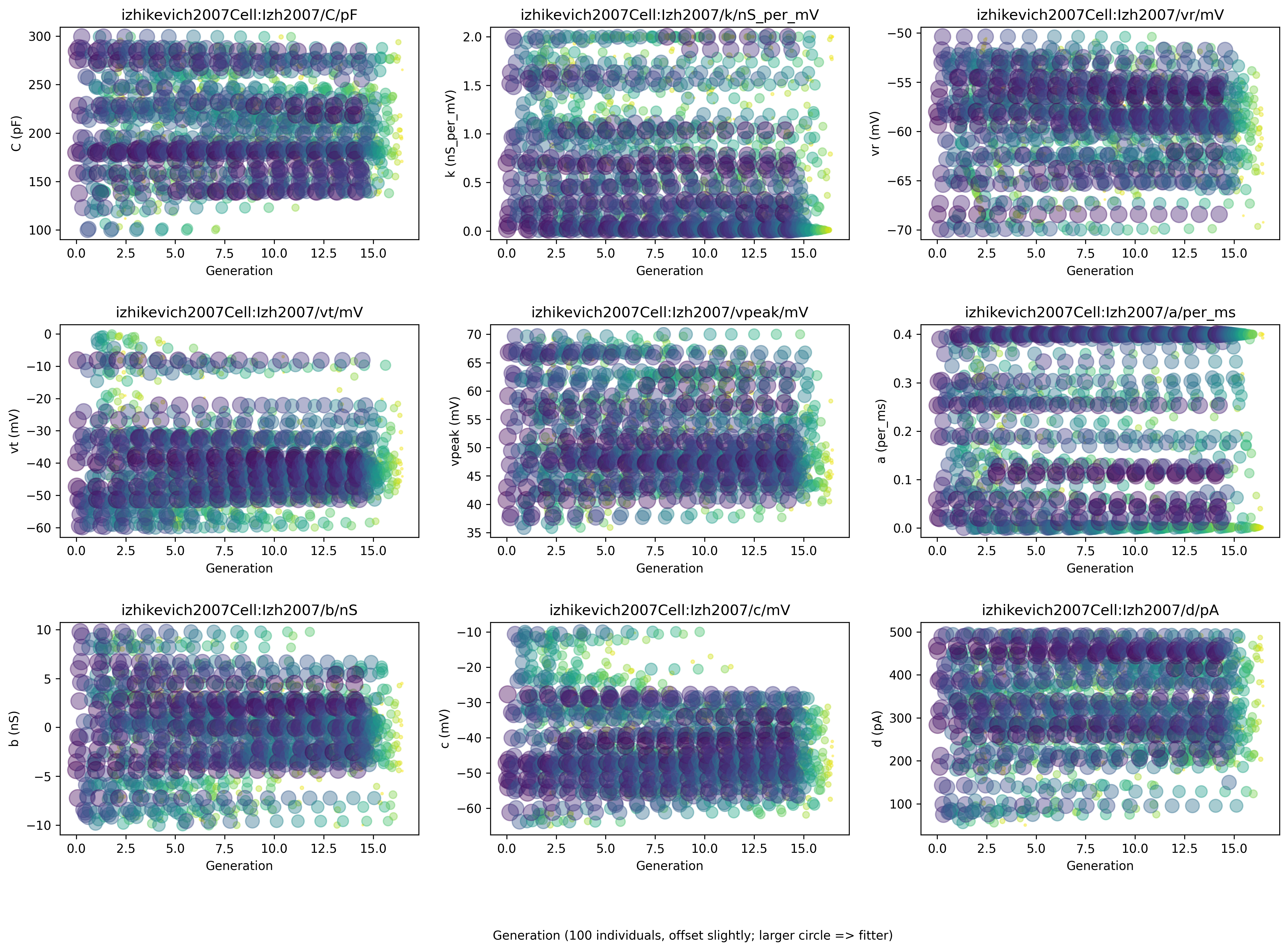
Fig. 48 The figure shows the values of various parameters throughout the evolution, with larger circles having higher values of fitness.#
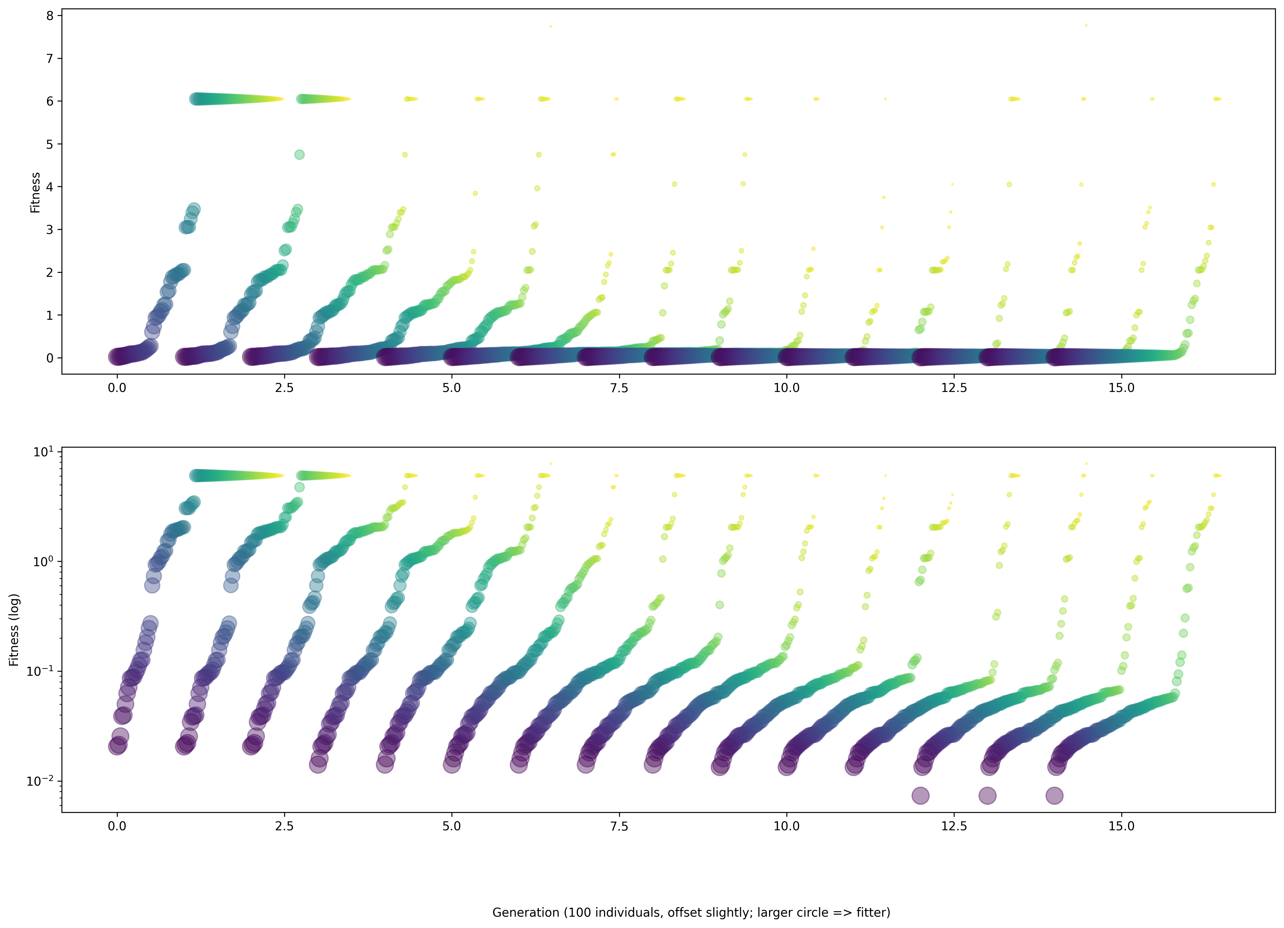
Fig. 49 The figure shows the trend of the fitness throughout the evolution.#
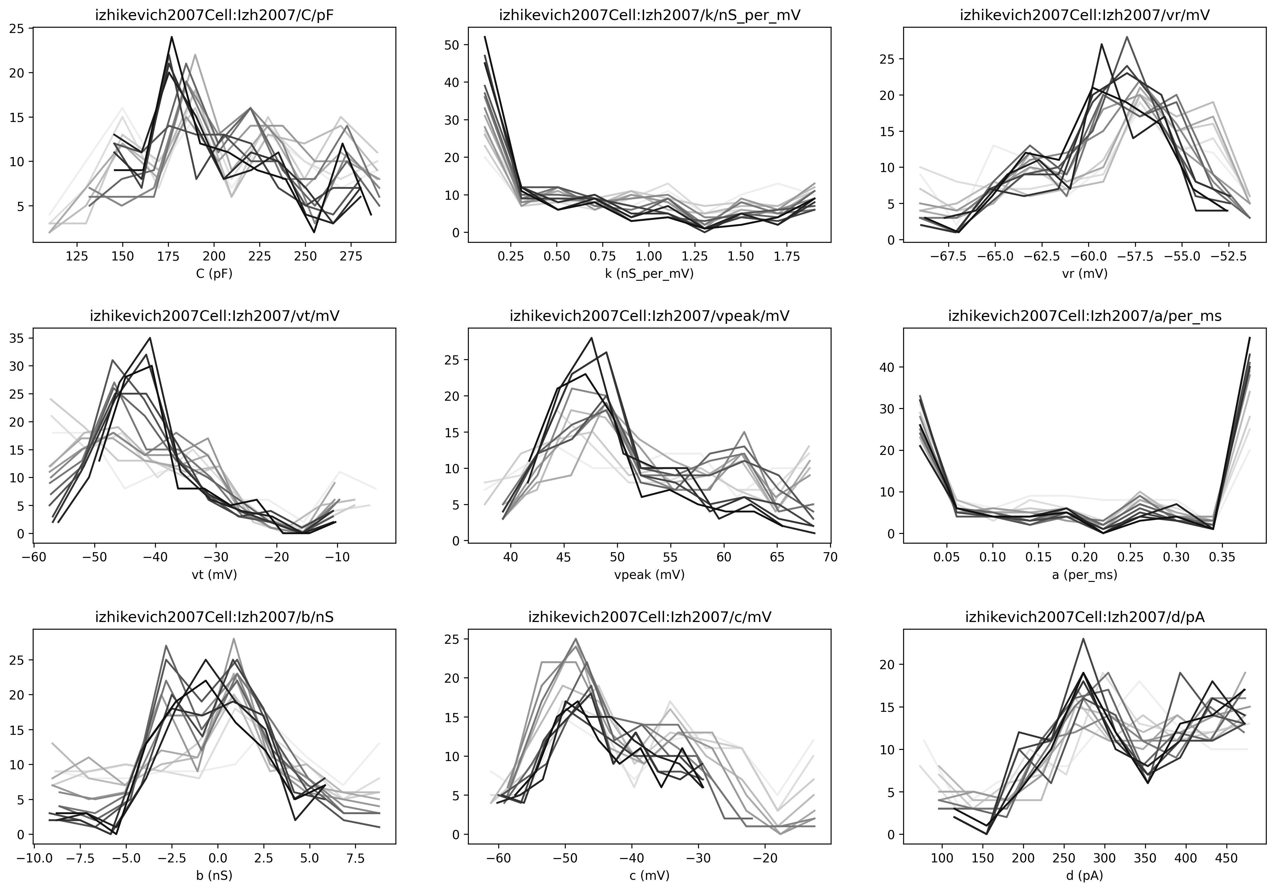
Fig. 50 The figure shows the distribution of values that for each parameter throughout the evolution. Darker lines have higher fitness values.#
Viewing results#
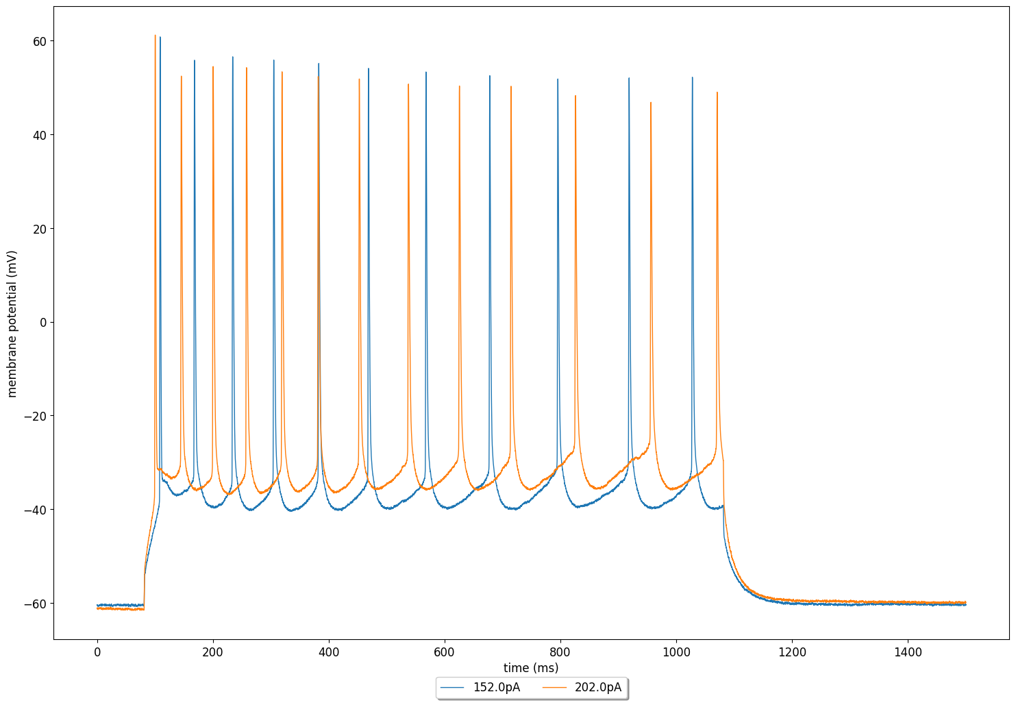
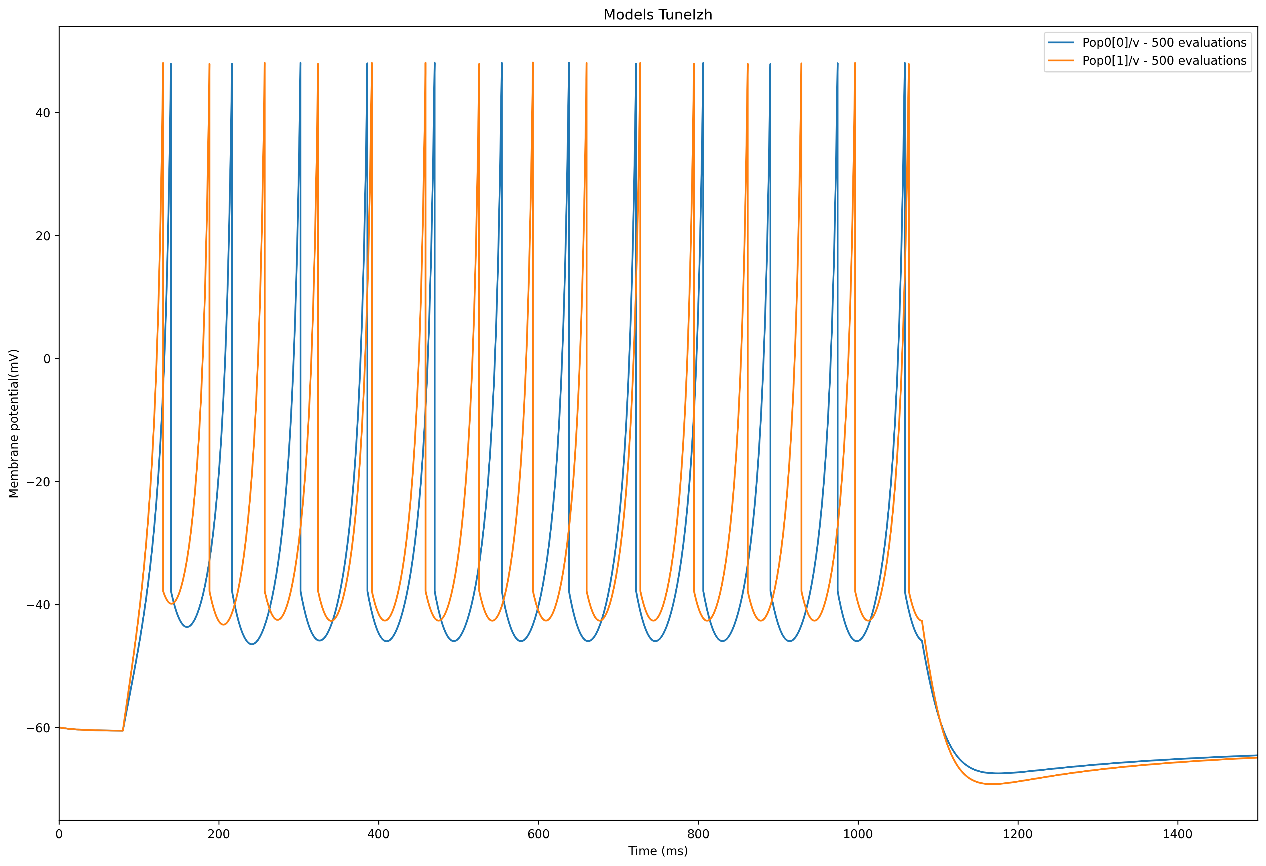
The tuner also generates a plot with the membrane potential of a cell using the fitted parameter values (shown on the top of the page).
Here, to document how the fitted parameters are to be extracted from the output of the run_optimisation function, we also construct a model to use the fitted parameters ourselves and plot the membrane potential to compare it against the experimental data.
Extracting results and running a fitted model#
This is done in the run_fitted_cell_simulation function:
def run_fitted_cell_simulation(
    sweeps_to_tune_against: List, tuning_report: Dict, simulation_id: str
) -> None:
    """Run a simulation with the values obtained from the fitting

    :param tuning_report: tuning report from the optimser
    :type tuning_report: Dict
    :param simulation_id: text id of simulation
    :type simulation_id: str

    """
    # get the fittest variables
    fittest_vars = tuning_report["fittest vars"]
    C = str(fittest_vars["izhikevich2007Cell:Izh2007/C/pF"]) + "pF"
    k = str(fittest_vars["izhikevich2007Cell:Izh2007/k/nS_per_mV"]) + "nS_per_mV"
    vr = str(fittest_vars["izhikevich2007Cell:Izh2007/vr/mV"]) + "mV"
    vt = str(fittest_vars["izhikevich2007Cell:Izh2007/vt/mV"]) + "mV"
    vpeak = str(fittest_vars["izhikevich2007Cell:Izh2007/vpeak/mV"]) + "mV"
    a = str(fittest_vars["izhikevich2007Cell:Izh2007/a/per_ms"]) + "per_ms"
    b = str(fittest_vars["izhikevich2007Cell:Izh2007/b/nS"]) + "nS"
    c = str(fittest_vars["izhikevich2007Cell:Izh2007/c/mV"]) + "mV"
    d = str(fittest_vars["izhikevich2007Cell:Izh2007/d/pA"]) + "pA"

    # Create a simulation using our obtained parameters.
    # Note that the tuner generates a graph with the fitted values already, but
    # we want to keep a copy of our fitted cell also, so we'll create a NeuroML
    # Document ourselves also.
    sim_time = 1500.0
    simulation_doc = NeuroMLDocument(id="FittedNet")
    # Add an Izhikevich cell with some parameters to the document
    simulation_doc.izhikevich2007_cells.append(
        Izhikevich2007Cell(
            id="Izh2007",
            C=C,
            v0="-60mV",
            k=k,
            vr=vr,
            vt=vt,
            vpeak=vpeak,
            a=a,
            b=b,
            c=c,
            d=d,
        )
    )
    simulation_doc.networks.append(Network(id="Network0"))
    # Add a cell for each acquisition list
    popsize = len(sweeps_to_tune_against)
    simulation_doc.networks[0].populations.append(
        Population(id="Pop0", component="Izh2007", size=popsize)
    )

    # Add a current source for each cell, matching the currents that
    # were used in the experimental study.
    counter = 0
    for acq in sweeps_to_tune_against:
        simulation_doc.pulse_generators.append(
            PulseGenerator(
                id="Stim{}".format(counter),
                delay="80ms",
                duration="1000ms",
                amplitude="{}pA".format(currents[acq]),
            )
        )
        simulation_doc.networks[0].explicit_inputs.append(
            ExplicitInput(
                target="Pop0[{}]".format(counter), input="Stim{}".format(counter)
            )
        )
        counter = counter + 1

    # Print a summary
    print(simulation_doc.summary())

    # Write to a neuroml file and validate it.
    reference = "FittedIzhFergusonPyr3"
    simulation_filename = "{}.net.nml".format(reference)
    write_neuroml2_file(simulation_doc, simulation_filename, validate=True)

    simulation = LEMSSimulation(
        sim_id=simulation_id,
        duration=sim_time,
        dt=0.1,
        target="Network0",
        simulation_seed=54321,
    )
    simulation.include_neuroml2_file(simulation_filename)
    simulation.create_output_file("output0", "{}.v.dat".format(simulation_id))
    counter = 0
    for acq in sweeps_to_tune_against:
        simulation.add_column_to_output_file(
            "output0", "Pop0[{}]".format(counter), "Pop0[{}]/v".format(counter)
        )
        counter = counter + 1
    simulation_file = simulation.save_to_file()
    # simulate
    run_lems_with_jneuroml(simulation_file, max_memory="2G", nogui=True, plot=False)
First, we extract the fitted parameters from the dictionary returned by the run_optimisation function.
Then, we use these parameters to set up a simple NeuroML network and run a test simulation, recording the values of membrane potentials generated by the cells.
Please note that the current stimulus to the cells in this test model must also match the values that were used in the experiment, and so also in the fitting.
Plotting model generated and experimentally recorded membrane potentials#
Finally, in the plot_sim_data function, we plot the membrane potentials from our fitted cells and the experimental data to see visually inspect the results of our fitting:
def plot_sim_data(
    sweeps_to_tune_against: List, simulation_id: str, memb_pots: Dict
) -> None:
    """Plot data from our fitted simulation

    :param simulation_id: string id of simulation
    :type simulation_id: str
    """
    # Plot
    data_array = np.loadtxt("%s.v.dat" % simulation_id)

    # construct data for plotting
    counter = 0
    time_vals_list = []
    sim_v_list = []
    data_v_list = []
    data_t_list = []
    stim_vals = []
    for acq in sweeps_to_tune_against:
        stim_vals.append("{}pA".format(currents[acq]))

        # remains the same for all columns
        time_vals_list.append(data_array[:, 0] * 1000.0)
        sim_v_list.append(data_array[:, counter + 1] * 1000.0)

        data_v_list.append(memb_pots[acq][1])
        data_t_list.append(memb_pots[acq][0])

        counter = counter + 1

    # Model membrane potential plot
    generate_plot(
        xvalues=time_vals_list,
        yvalues=sim_v_list,
        labels=stim_vals,
        title="Membrane potential (model)",
        show_plot_already=False,
        save_figure_to="%s-model-v.png" % simulation_id,
        xaxis="time (ms)",
        yaxis="membrane potential (mV)",
    )
    # data membrane potential plot
    generate_plot(
        xvalues=data_t_list,
        yvalues=data_v_list,
        labels=stim_vals,
        title="Membrane potential (exp)",
        show_plot_already=False,
        save_figure_to="%s-exp-v.png" % simulation_id,
        xaxis="time (ms)",
        yaxis="membrane potential (mV)",
    )
This generates the following figures:
We can clearly see the similarity between our fitted model and the experimental data. A number of tweaks can be made to improve the fitting. For example, pyNeuroML also provides a two staged optimisation function: run_2stage_optimisation that allows users to optimise sets of parameters in two different stages. The graphs also show ranges of parameters that provide fits, so users can also hand-tune their models further as required.