Visualising NeuroML Models#
A number of the NeuroML software tools can be used to easily visualise models described in NeuroML.
Get a quick summary of your model#
Using command line tools#
You can get a quick summary of your NeuroML model using the pynml-summary command line tool that is provided by pyNeuroML:
Usage:
pynml-summary <NeuroML file>
For example, to get a quick summary of the Primary Auditory Cortex model by Dave Beeman (see it here on Open Source Brain), one can run:
pynml-summary MediumNet.net.nml

*******************************************************
* NeuroMLDocument: network_ACnet2
*
*  PulseGenerator: ['BackgroundRandomIClamps']
*
*  Network: network_ACnet2 (temperature: 6.3 degC)
*
*   60 cells in 2 populations
*     Population: baskets_12 with 12 components of type bask
*       Locations: [(372.5585, 75.3425, 459.2106), ...]
*       Properties: color=0.0 0.19921875 0.59765625;
*     Population: pyramidals_48 with 48 components of type pyr_4_sym
*       Locations: [(64.2564, 0.6838, 94.8305), ...]
*       Properties: color=0.796875 0.0 0.0;
*
*   984 connections in 4 projections
*     Projection: SmallNet_bask_bask from baskets_12 to baskets_12, synapse: GABA_syn_inh
*       60 connections: [(Connection 0: 3:0(0.41661) -> 0:0(0.68577)), ...]
*     Projection: SmallNet_bask_pyr from baskets_12 to pyramidals_48, synapse: GABA_syn
*       336 connections: [(Connection 0: 10:0(0.05824) -> 0:6(0.02628)), ...]
*     Projection: SmallNet_pyr_bask from pyramidals_48 to baskets_12, synapse: AMPA_syn_inh
*       252 connections: [(Connection 0: 1:0(0.89734) -> 0:1(0.09495)), ...]
*     Projection: SmallNet_pyr_pyr from pyramidals_48 to pyramidals_48, synapse: AMPA_syn
*       336 connections: [(Connection 0: 14:0(0.52814) -> 0:3(0.10797)), ...]
*
*   14 inputs in 1 input lists
*     Input list: BackgroundRandomIClamps to pyramidals_48, component BackgroundRandomIClamps
*       14 inputs: [(Input 0: 37:0(0.500000)), ...]
*
*******************************************************
Using pyNeuroML#
You can also get a summary of your model from within your pyNeuroML script itself using the summary function:
import pyneuroml.pynml

...


pyneuroml.pynml.summary(nml2_doc)
View the 3D structure of your model#
Using command line tools#
You can generate an image of the 3D structure of the NeuroML model using the pynml command provided by pyNeuroML, or using the jnml command provided by jNeuroML:
Usage:
pynml -png/-svg <NeuroML file>
jnml -png/-svg <NeuroML file>
For example, to generate a PNG image of the Auditory Cortex model used above, we can use (use -svg to generate a vectorised SVG image instead of a PNG):
pynml -png MediumNet.net.nml
This generates the following image showing different views of the network :
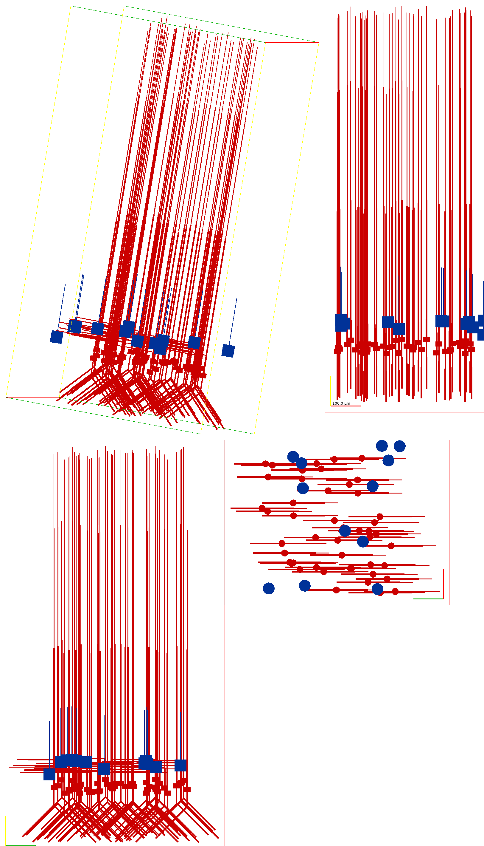
Fig. 31 Graphical view of the Auditory Cortex model generated with pynml#
An visualiser is also included in pyneuroml as pynml-plotmorph which includes both 2D and 3D views:
Usage:
pynml-plotmorph <NeuroML file>
pynml-plotmorph -i <NeuroML file>
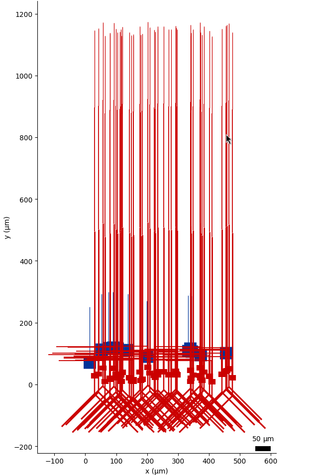
Fig. 32 Matplotlib based 2D visualisation of a network with pynml-plotmorph.#
Example network visualised interactively using `pynml-plotmorph`
You can also generate graphical representations that can be viewed with the Persistence of Vision Raytracer (POV-Ray) tool using the pynml-povray tool.
For example:
pynml-povray MediumNet.net.nml -scalez 8
povray Antialias=On Antialias_Depth=10 Antialias_Threshold=0.1 Output_to_File=y Output_File_Type=N Output_File_Name=Acnet-medium.povray +W1200 +H900 MediumNet.net.nml.pov
generates this image:
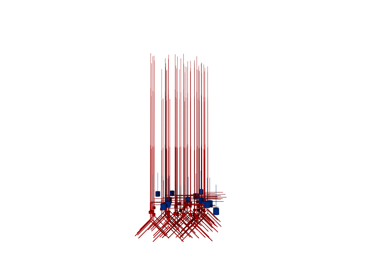
Fig. 33 Graphical view of the Auditory Cortex model generated with pynml-povray and POV-Ray#
You can also use POV-Ray interactively.
Please refer to the official website for more information on installing and using POV-Ray.
On Fedora Linux systems, you can install it from the Fedora repositories using dnf:
sudo dnf install povray
Using pyNeuroML#
These functions are also exposed as Python functions in pyNeuroML, so that you can use them directly in Python scripts:
import pyneuroml.pynml

pyneuroml.pynml.nml2_to_png(nml2_doc)
pyneuroml.pynml.nml2_to_svg(nml2_doc)


from pyneuroml.plot.PlotMorphology import plot_2D
from pyneuroml.plot.PlotMorphologyVispy import plot_interactive_3D

plot_2D(nml2_doc)
plot_interactive_3D(nml2_doc)
Open Source Brain uses NeuroML.
The Open Source Brain platform generates the interactive visualisations from NeuroML sources. See the Auditory Cortex model on Open Source Brain here.
View the connectivity graph of your model#
Using command line tools#
Use levels to generate connectivity graphs with different levels of detail.
Positive values for levels will generate figures at the population level, while negative values will generate them at the level of cells.
You can generate an image of the 3D structure of the NeuroML model using pynml:
Usage:
pynml <NeuroML file> -graph <level, engine>
For example, to generate a PNG image of the Auditory Cortex model used above, we can use:
pynml MediumNet.net.nml -graph 1d
This generates the following image showing different views of the network :

Fig. 34 Level 1 network graph generated by pynml#
You can modify the level of detail included in the graph by using different values of levels. For example, this command generates a level 5 graph:
pynml MediumNet.net.nml -graph 5d
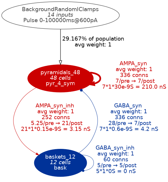
Fig. 35 Level 5 network graph generated by pynml#
Using pyNeuroML#
You can also generated these figures from within your pyNeuroML script itself using the generate_nmlgraph function:
import pyneuroml.pynml

...


pyneuroml.pynml.generate_nmlgraph(nml2_doc, level="1", engine="dot")
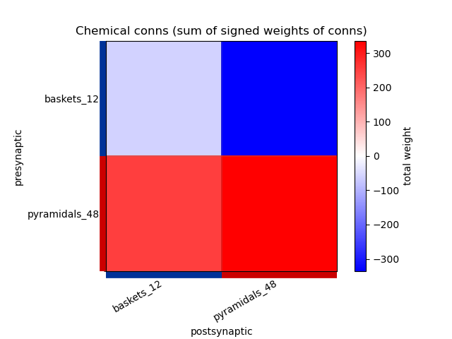
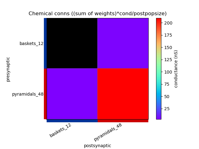
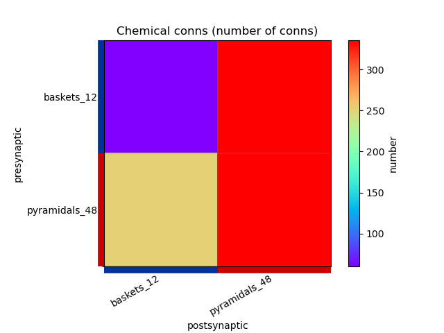
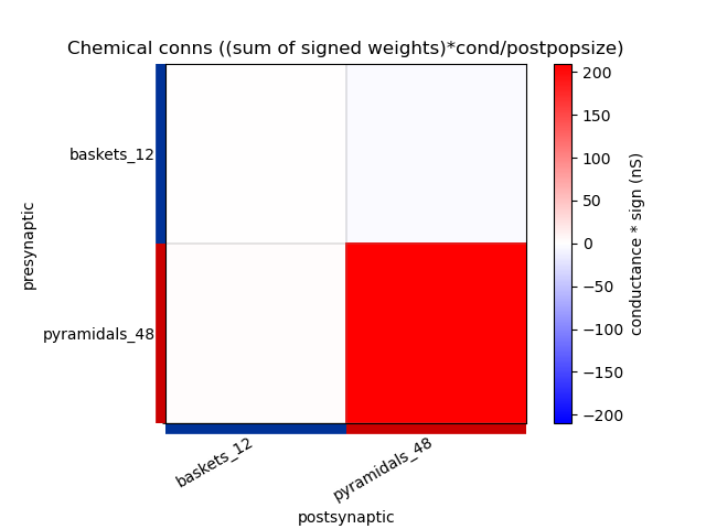
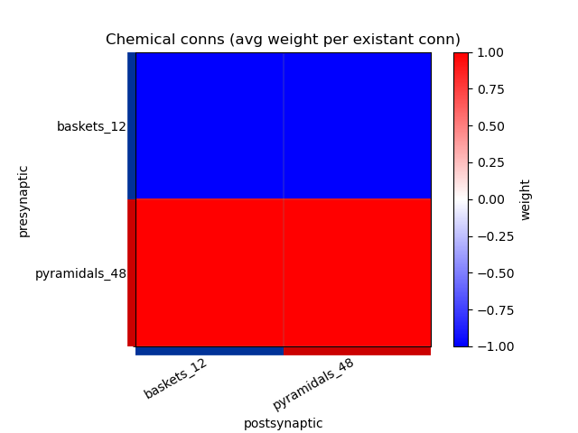
View the connectivity matrices of the model#
You can generate the connectivity matrices of projections between neuronal populations of the NeuroML model using pynml:
Usage:
pynml <NeuroML file> -matrix <level>
For example, to generate a PNG image of the connectivity matrices in the Auditory Cortex model used above, we can use:
pynml MediumNet.net.nml -matrix 1
This generates the following images showing different views of the connectivity matrices in the network :
View graph of the simulation instance of the model#
Using command line tools#
When you have created a simulation instance of the NeuroML model using LEMS, you can also visualise this using pynml or jnml:
Usage:
pynml <LEMS simulation file> -lems-graph
jnml <LEMS simulation file> -lems-graph
For example, to generate the LEMS graph for the Izhikevich neuron network example, we will use:
jnml LEMS_example_izhikevich2007network_sim.xml -lems-graph
will generate:
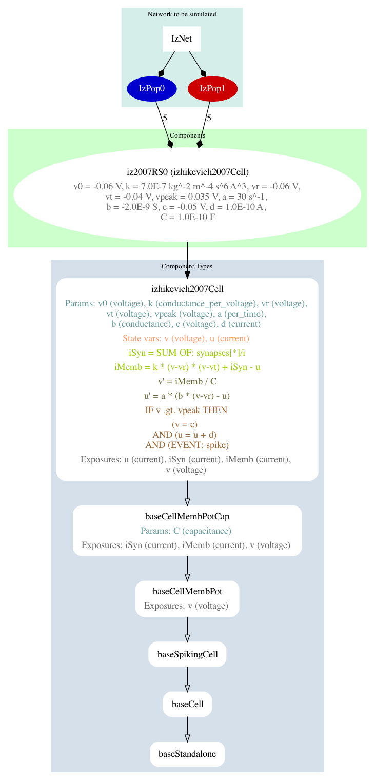
Fig. 36 A summary graph of the model generated using jnml.#
Note that the -lems-graph option does not take options for levels of detail.
It shows all the details of the simulation instance, and so is better suited for simpler models rather than detailed conductance based network models.
For example, for the Auditory Cortex model, this very very detailed image is generated (please click to open: it is too large to display in the page).
Using pyNeuroML#
You can also generated these figures from within your pyNeuroML script itself using the generate_lemsgraph function:
import pyneuroml.pynml

...

pyneuroml.pynml.generate_lemsgraph(lems_file)
Viewing/analysing ion channel dynamics#
There is a dedicated section on visualising and analysing ion channel models.