A two population network of regular spiking Izhikevich neurons

Now that we have defined a cell, let us see how a network of these cells may be declared and simulated. We will create a small network of cells, simulate this network, and generate a plot of the spike times of the cells (a raster plot):

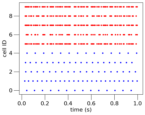
Fig. 9 Spike times of neurons in 2 populations recorded from the simulation.

The Python script used to create the model, simulate it, and generate this plot is below. Please note that this example uses the NEURON simulator to simulate the model. Please ensure that the NEURON_HOME environment variable is correctly set as noted here.

#!/usr/bin/env python3
"""
Create a simple network with two populations.
"""

import random
import numpy as np

from neuroml.utils import component_factory
from pyneuroml import pynml
from pyneuroml.lems import LEMSSimulation
import neuroml.writers as writers


nml_doc = component_factory("NeuroMLDocument", id="IzNet")
iz0 = nml_doc.add(
    "Izhikevich2007Cell",
    id="iz2007RS0",
    v0="-60mV",
    C="100pF",
    k="0.7nS_per_mV",
    vr="-60mV",
    vt="-40mV",
    vpeak="35mV",
    a="0.03per_ms",
    b="-2nS",
    c="-50.0mV",
    d="100pA",
)

# Inspect the component, also show all members:
iz0.info(True)

# Create a component of type ExpOneSynapse, and add it to the document
syn0 = nml_doc.add(
    "ExpOneSynapse", id="syn0", gbase="65nS", erev="0mV", tau_decay="3ms"
)
# Check what we have so far:
nml_doc.info(True)
# Also try:
print(nml_doc.summary())

# create the network: turned of validation because we will add populations next
net = nml_doc.add("Network", id="IzNet", validate=False)

# create the first population
size0 = 5
pop0 = component_factory("Population", id="IzPop0", component=iz0.id, size=size0)
# Set optional color property. Note: used later when generating plots
pop0.add("Property", tag="color", value="0 0 .8")
net.add(pop0)

# create the second population
size1 = 5
pop1 = component_factory("Population", id="IzPop1", component=iz0.id, size=size1)
pop1.add("Property", tag="color", value=".8 0 0")
net.add(pop1)

# network should be valid now that it contains populations
net.validate()

# create a projection from one population to another
proj = net.add(
    "Projection",
    id="proj",
    presynaptic_population=pop0.id,
    postsynaptic_population=pop1.id,
    synapse=syn0.id,
)

# We do two things in the loop:
# - add pulse generator inputs to population 1 to make neurons spike
# - create synapses between the two populations with a particular probability
random.seed(123)
prob_connection = 0.8
count = 0
for pre in range(0, size0):
    # pulse generator as explicit stimulus
    pg = nml_doc.add(
        "PulseGenerator",
        id="pg_%i" % pre,
        delay="0ms",
        duration="10000ms",
        amplitude="%f nA" % (0.1 + 0.1 * random.random()),
    )

    exp_input = net.add(
        "ExplicitInput", target="%s[%i]" % (pop0.id, pre), input=pg.id
    )

    # synapses between populations
    for post in range(0, size1):
        if random.random() <= prob_connection:
            syn = proj.add(
                "Connection",
                id=count,
                pre_cell_id="../%s[%i]" % (pop0.id, pre),
                post_cell_id="../%s[%i]" % (pop1.id, post),
            )
            count += 1

nml_doc.info(True)
print(nml_doc.summary())

# write model to file and validate
nml_file = "izhikevich2007_network.nml"
writers.NeuroMLWriter.write(nml_doc, nml_file)

print("Written network file to: " + nml_file)
pynml.validate_neuroml2(nml_file)

# Create simulation, and record data
simulation_id = "example_izhikevich2007network_sim"
simulation = LEMSSimulation(
    sim_id=simulation_id, duration=1000, dt=0.1, simulation_seed=123
)
simulation.assign_simulation_target(net.id)
simulation.include_neuroml2_file(nml_file)

simulation.create_event_output_file(
    "pop0", "%s.0.spikes.dat" % simulation_id, format="ID_TIME"
)
for pre in range(0, size0):
    simulation.add_selection_to_event_output_file(
        "pop0", pre, "IzPop0[{}]".format(pre), "spike"
    )

simulation.create_event_output_file(
    "pop1", "%s.1.spikes.dat" % simulation_id, format="ID_TIME"
)
for pre in range(0, size1):
    simulation.add_selection_to_event_output_file(
        "pop1", pre, "IzPop1[{}]".format(pre), "spike"
    )

lems_simulation_file = simulation.save_to_file()

# Run the simulation
pynml.run_lems_with_jneuroml_neuron(
    lems_simulation_file, max_memory="2G", nogui=True, plot=False
)

# Load the data from the file and plot the spike times
# using the pynml generate_plot utility function.
data_array_0 = np.loadtxt("%s.0.spikes.dat" % simulation_id)
data_array_1 = np.loadtxt("%s.1.spikes.dat" % simulation_id)
times_0 = data_array_0[:, 1]
times_1 = data_array_1[:, 1]
ids_0 = data_array_0[:, 0]
ids_1 = [id + size0 for id in data_array_1[:, 0]]
pynml.generate_plot(
    [times_0, times_1],
    [ids_0, ids_1],
    "Spike times",
    show_plot_already=False,
    save_figure_to="%s-spikes.png" % simulation_id,
    xaxis="time (s)",
    yaxis="cell ID",
    colors=["b", "r"],
    linewidths=["0", "0"],
    markers=[".", "."],
)

As with the previous example, we will step through this script to see how the various components of the network are declared in NeuroML before running the simulation and generating the plot. We will use the same helper functions to inspect the model as we build it: component_factory, add, info, summary.

Declaring the model in NeuroML

To declare the complete network model, we must again first declare its core entities:

nml_doc = component_factory("NeuroMLDocument", id="IzNet")
iz0 = nml_doc.add(
    "Izhikevich2007Cell",
    id="iz2007RS0",
    v0="-60mV",
    C="100pF",
    k="0.7nS_per_mV",
    vr="-60mV",
    vt="-40mV",
    vpeak="35mV",
    a="0.03per_ms",
    b="-2nS",
    c="-50.0mV",
    d="100pA",
)

# Inspect the component, also show all members:
iz0.info(True)

# Create a component of type ExpOneSynapse, and add it to the document
syn0 = nml_doc.add(
    "ExpOneSynapse", id="syn0", gbase="65nS", erev="0mV", tau_decay="3ms"
)

Here, we create a new document, declare the Izhikevich neuron, and also declare the synapse that we are going to use to connect one population of neurons to the other. We use the ExpOne Synapse here, where the conductance of the synapse increases instantaneously by a constant value gbase on receiving a spike, and then decays exponentially with a decay constant tauDecay.

Let’s inspect our model document so far:

nml_doc.info(True)
Please see the NeuroML standard schema documentation at https://docs.neuroml.org/Userdocs/NeuroMLv2.html for more information.

Valid members for NeuroMLDocument are:
...
* izhikevich2007_cells (class: Izhikevich2007Cell, Optional)
        * Contents ('ids'/<objects>): ['iz2007RS0']

* ad_ex_ia_f_cells (class: AdExIaFCell, Optional)
* fitz_hugh_nagumo_cells (class: FitzHughNagumoCell, Optional)
* fitz_hugh_nagumo1969_cells (class: FitzHughNagumo1969Cell, Optional)
* pinsky_rinzel_ca3_cells (class: PinskyRinzelCA3Cell, Optional)
* pulse_generators (class: PulseGenerator, Optional)
* pulse_generator_dls (class: PulseGeneratorDL, Optional)
* id (class: NmlId, Required)
        * Contents ('ids'/<objects>): IzNet

* sine_generators (class: SineGenerator, Optional)
...
* IF_curr_exp (class: IF_curr_exp, Optional)
* exp_one_synapses (class: ExpOneSynapse, Optional)
        * Contents ('ids'/<objects>): ['syn0']

* IF_cond_alpha (class: IF_cond_alpha, Optional)
* exp_two_synapses (class: ExpTwoSynapse, Optional)
...

Let’s also get a summary:

print(nml_doc.summary())
*******************************************************
* NeuroMLDocument: IzNet
*
*  ExpOneSynapse: ['syn0']
*  Izhikevich2007Cell: ['iz2007RS0']
*
*******************************************************

We can now declare our network with 2 populations of these cells. Note: setting a color as a property is optional, but is used in when we generate our plots below.

# create the network: turned of validation because we will add populations next
net = nml_doc.add("Network", id="IzNet", validate=False)

# create the first population
size0 = 5
pop0 = component_factory("Population", id="IzPop0", component=iz0.id, size=size0)
# Set optional color property. Note: used later when generating plots
pop0.add("Property", tag="color", value="0 0 .8")
net.add(pop0)

# create the second population
size1 = 5
pop1 = component_factory("Population", id="IzPop1", component=iz0.id, size=size1)
pop1.add("Property", tag="color", value=".8 0 0")
net.add(pop1)

We can test to see if the network is now valid, since we have added the required populations to it:

net.validate()

This function does not return anything if the component is valid. If it is invalid, however, it will throw a ValueError.

We can now create projections between the two populations based on some probability of connection. To do this, we iterate over each post-synaptic neuron for each pre-synaptic neuron and draw a random number between 0 and 1. If the drawn number is less than the required probability of connection, the connection is created.

While we are iterating over all our pre-synaptic cells here, we also add external inputs to them using ExplicitInputs (this could have been done in a different loop, but it is convenient to also do this here).

# create a projection from one population to another
proj = net.add(
    "Projection",
    id="proj",
    presynaptic_population=pop0.id,
    postsynaptic_population=pop1.id,
    synapse=syn0.id,
)

# We do two things in the loop:
# - add pulse generator inputs to population 1 to make neurons spike
# - create synapses between the two populations with a particular probability
random.seed(123)
prob_connection = 0.8
count = 0
for pre in range(0, size0):
    # pulse generator as explicit stimulus
    pg = nml_doc.add(
        "PulseGenerator",
        id="pg_%i" % pre,
        delay="0ms",
        duration="10000ms",
        amplitude="%f nA" % (0.1 + 0.1 * random.random()),
    )

    exp_input = net.add(
        "ExplicitInput", target="%s[%i]" % (pop0.id, pre), input=pg.id
    )

    # synapses between populations
    for post in range(0, size1):
        if random.random() <= prob_connection:
            syn = proj.add(
                "Connection",
                id=count,
                pre_cell_id="../%s[%i]" % (pop0.id, pre),
                post_cell_id="../%s[%i]" % (pop1.id, post),
            )
            count += 1

Let us inspect our model again to confirm that we have it set up correctly.

nml_doc.info(True)
Please see the NeuroML standard schema documentation at https://docs.neuroml.org/Userdocs/NeuroMLv2.html for more information.

Valid members for NeuroMLDocument are:
* biophysical_properties (class: BiophysicalProperties, Optional)
* SpikeSourcePoisson (class: SpikeSourcePoisson, Optional)
* cells (class: Cell, Optional)
* networks (class: Network, Optional)
        * Contents ('ids'/<objects>): ['IzNet']

* cell2_ca_poolses (class: Cell2CaPools, Optional)
...
* izhikevich2007_cells (class: Izhikevich2007Cell, Optional)
        * Contents ('ids'/<objects>): ['iz2007RS0']

* ad_ex_ia_f_cells (class: AdExIaFCell, Optional)
* fitz_hugh_nagumo_cells (class: FitzHughNagumoCell, Optional)
* fitz_hugh_nagumo1969_cells (class: FitzHughNagumo1969Cell, Optional)
* pinsky_rinzel_ca3_cells (class: PinskyRinzelCA3Cell, Optional)
* pulse_generators (class: PulseGenerator, Optional)
        * Contents ('ids'/<objects>): ['pg_0', 'pg_1', 'pg_2', 'pg_3', 'pg_4']

* pulse_generator_dls (class: PulseGeneratorDL, Optional)
* id (class: NmlId, Required)
        * Contents ('ids'/<objects>): IzNet

...
* exp_one_synapses (class: ExpOneSynapse, Optional)
        * Contents ('ids'/<objects>): ['syn0']

* IF_cond_alpha (class: IF_cond_alpha, Optional)
..


print(nml_doc.summary())
*******************************************************
* NeuroMLDocument: IzNet
*
*  ExpOneSynapse: ['syn0']
*  Izhikevich2007Cell: ['iz2007RS0']
*  PulseGenerator: ['pg_0', 'pg_1', 'pg_2', 'pg_3', 'pg_4']
*
*  Network: IzNet
*
*   10 cells in 2 populations
*     Population: IzPop0 with 5 components of type iz2007RS0
*       Properties: color=0 0 .8;
*     Population: IzPop1 with 5 components of type iz2007RS0
*       Properties: color=.8 0 0;
*
*   20 connections in 1 projections
*     Projection: proj from IzPop0 to IzPop1, synapse: syn0
*       20 connections: [(Connection 0: 0 -> 0), ...]
*
*   0 inputs in 0 input lists
*
*   5 explicit inputs (outside of input lists)
*     Explicit Input of type pg_0 to IzPop0(cell 0), destination: unspecified
*     Explicit Input of type pg_1 to IzPop0(cell 1), destination: unspecified
*     Explicit Input of type pg_2 to IzPop0(cell 2), destination: unspecified
*     Explicit Input of type pg_3 to IzPop0(cell 3), destination: unspecified
*     Explicit Input of type pg_4 to IzPop0(cell 4), destination: unspecified
*
*******************************************************

We can now save and validate our model.

# write model to file and validate
nml_file = "izhikevich2007_network.nml"
writers.NeuroMLWriter.write(nml_doc, nml_file)

print("Written network file to: " + nml_file)
pynml.validate_neuroml2(nml_file)

The generated NeuroML model

Let us take a look at the generated NeuroML model

<neuroml xmlns="http://www.neuroml.org/schema/neuroml2"  xmlns:xs="http://www.w3.org/2001/XMLSchema" xmlns:xsi="http://www.w3.org/2001/XMLSchema-instance" xsi:schemaLocation="http://www.neuroml.org/schema/neuroml2 https://raw.github.com/NeuroML/NeuroML2/development/Schemas/NeuroML2/NeuroML_v2.3.xsd" id="IzNet">
    <expOneSynapse id="syn0" gbase="65nS" erev="0mV" tauDecay="3ms"/>
    <izhikevich2007Cell id="iz2007RS0" C="100pF" v0="-60mV" k="0.7nS_per_mV" vr="-60mV" vt="-40mV" vpeak="35mV" a="0.03per_ms" b="-2nS" c="-50.0mV" d="100pA"/>
    <pulseGenerator id="pg_0" delay="0ms" duration="10000ms" amplitude="0.105236 nA"/>
    <pulseGenerator id="pg_1" delay="0ms" duration="10000ms" amplitude="0.153620 nA"/>
    <pulseGenerator id="pg_2" delay="0ms" duration="10000ms" amplitude="0.124516 nA"/>
    <pulseGenerator id="pg_3" delay="0ms" duration="10000ms" amplitude="0.131546 nA"/>
    <pulseGenerator id="pg_4" delay="0ms" duration="10000ms" amplitude="0.102124 nA"/>
    <network id="IzNet">
        <population id="IzPop0" component="iz2007RS0" size="5" type="population">
            <property tag="color" value="0 0 .8"/>
        </population>
        <population id="IzPop1" component="iz2007RS0" size="5" type="population">
            <property tag="color" value=".8 0 0"/>
        </population>
        <projection id="proj" presynapticPopulation="IzPop0" postsynapticPopulation="IzPop1" synapse="syn0">
            <connection id="0" preCellId="../IzPop0[0]" postCellId="../IzPop1[0]"/>
            <connection id="1" preCellId="../IzPop0[0]" postCellId="../IzPop1[1]"/>
            <connection id="2" preCellId="../IzPop0[0]" postCellId="../IzPop1[2]"/>
            <connection id="3" preCellId="../IzPop0[0]" postCellId="../IzPop1[4]"/>
            <connection id="4" preCellId="../IzPop0[1]" postCellId="../IzPop1[0]"/>
            <connection id="5" preCellId="../IzPop0[1]" postCellId="../IzPop1[2]"/>
            <connection id="6" preCellId="../IzPop0[1]" postCellId="../IzPop1[3]"/>
            <connection id="7" preCellId="../IzPop0[1]" postCellId="../IzPop1[4]"/>
            <connection id="8" preCellId="../IzPop0[2]" postCellId="../IzPop1[0]"/>
            <connection id="9" preCellId="../IzPop0[2]" postCellId="../IzPop1[1]"/>
            <connection id="10" preCellId="../IzPop0[2]" postCellId="../IzPop1[2]"/>
            <connection id="11" preCellId="../IzPop0[2]" postCellId="../IzPop1[3]"/>
            <connection id="12" preCellId="../IzPop0[2]" postCellId="../IzPop1[4]"/>
            <connection id="13" preCellId="../IzPop0[3]" postCellId="../IzPop1[0]"/>
            <connection id="14" preCellId="../IzPop0[3]" postCellId="../IzPop1[2]"/>
            <connection id="15" preCellId="../IzPop0[3]" postCellId="../IzPop1[3]"/>
            <connection id="16" preCellId="../IzPop0[3]" postCellId="../IzPop1[4]"/>
            <connection id="17" preCellId="../IzPop0[4]" postCellId="../IzPop1[1]"/>
            <connection id="18" preCellId="../IzPop0[4]" postCellId="../IzPop1[2]"/>
            <connection id="19" preCellId="../IzPop0[4]" postCellId="../IzPop1[4]"/>
        </projection>
        <explicitInput target="IzPop0[0]" input="pg_0"/>
        <explicitInput target="IzPop0[1]" input="pg_1"/>
        <explicitInput target="IzPop0[2]" input="pg_2"/>
        <explicitInput target="IzPop0[3]" input="pg_3"/>
        <explicitInput target="IzPop0[4]" input="pg_4"/>
    </network>
</neuroml>

It should now be easy to see how the model is clearly declared in the NeuroML file. Observe how entities are referenced in NeuroML depending on their location in the document architecture. Here, population and projection are at the same level. The synaptic connections using the connection tag are at the next level. So, in the connection tags, populations are to be referred to as ../ which indicates the previous level. The explicitinput tag is at the same level as the population and projection tags, so we do not need to use ../ here to reference them.

Another point worth noting here is that because we have defined a population of the same components by specifying a size rather than by individually adding components to it, we can refer to the entities of the population using the common [..] index operator.

The advantage of such a declarative format is that we can also easily get information on our model from the NeuroML file. Similar to the summary() function that we have used so far, pyNeuroML also includes the helper pynml-summary script that can be used to get summaries of NeuroML models from their NeuroML files:

$ pynml-summary izhikevich2007_network.nml
*******************************************************
* NeuroMLDocument: IzNet
*
*   ExpOneSynapse: ['syn0']
*   Izhikevich2007Cell: ['iz2007RS0']
*   PulseGenerator: ['pulseGen_0', 'pulseGen_1', 'pulseGen_2', 'pulseGen_3', 'pulseGen_4']
*
*  Network: IzNet
*
*   10 cells in 2 populations
*     Population: IzPop0 with 5 components of type iz2007RS0
*     Population: IzPop1 with 5 components of type iz2007RS0
*
*   20 connections in 1 projections
*     Projection: proj from IzPop0 to IzPop1, synapse: syn0
*       20 connections: [(Connection 0: 0 -> 0), ...]
*
*   0 inputs in 0 input lists
*
*   5 explicit inputs (outside of input lists)
*     Explicit Input of type pulseGen_0 to IzPop0(cell 0), destination: unspecified
*     Explicit Input of type pulseGen_1 to IzPop0(cell 1), destination: unspecified
*     Explicit Input of type pulseGen_2 to IzPop0(cell 2), destination: unspecified
*     Explicit Input of type pulseGen_3 to IzPop0(cell 3), destination: unspecified
*     Explicit Input of type pulseGen_4 to IzPop0(cell 4), destination: unspecified
*
*******************************************************

We can also generate a graphical summary of our model using pynml from pyNeuroML:

$ pynml izhikevich2007_network.nml -graph 3

This generates the following model summary diagram:

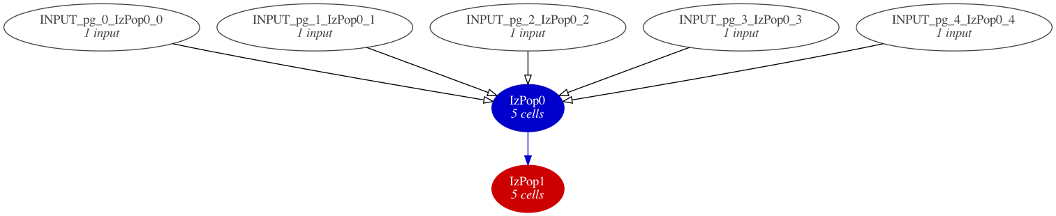
Fig. 10 A summary graph of the model generated using pynml and the dot tool.

Other options for pynml produce other views, e.g individual connections:

$ pynml izhikevich2007_network.nml -graph -1

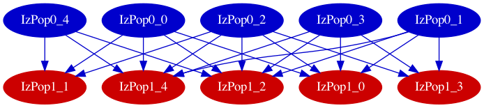
Fig. 11 Model summary graph showing individual connections between cells in the populations.

In our very simple network here, neurons do not have morphologies and are not distributed in space. In later examples, however, we will also see how summary figures of the network that show the morphologies, locations of different layers and neurons, and so on can also be generated using the NeuroML tools.

Simulating the model

Now that we have our model set up, we can proceed to simulating it. We create our simulation, and setup the information we want to record from it.

# Create simulation, and record data
simulation_id = "example_izhikevich2007network_sim"
simulation = LEMSSimulation(
    sim_id=simulation_id, duration=1000, dt=0.1, simulation_seed=123
)
simulation.assign_simulation_target(net.id)
simulation.include_neuroml2_file(nml_file)

simulation.create_event_output_file(
    "pop0", "%s.0.spikes.dat" % simulation_id, format="ID_TIME"
)
for pre in range(0, size0):
    simulation.add_selection_to_event_output_file(
        "pop0", pre, "IzPop0[{}]".format(pre), "spike"
    )

simulation.create_event_output_file(
    "pop1", "%s.1.spikes.dat" % simulation_id, format="ID_TIME"
)
for pre in range(0, size1):
    simulation.add_selection_to_event_output_file(
        "pop1", pre, "IzPop1[{}]".format(pre), "spike"
    )

lems_simulation_file = simulation.save_to_file()

The generated LEMS file is here:

<Lems>

    <!-- 

        This LEMS file has been automatically generated using PyNeuroML v1.1.13 (libNeuroML v0.5.8)

     -->

    <!-- Specify which component to run -->
    <Target component="example_izhikevich2007network_sim"/>

    <!-- Include core NeuroML2 ComponentType definitions -->
    <Include file="Cells.xml"/>
    <Include file="Networks.xml"/>
    <Include file="Simulation.xml"/>

    <Include file="izhikevich2007_network.nml"/>

    <Simulation id="example_izhikevich2007network_sim" length="1000ms" step="0.1ms" target="IzNet" seed="123">  <!-- Note seed: ensures same random numbers used every run -->
        <EventOutputFile id="pop0" fileName="example_izhikevich2007network_sim.0.spikes.dat" format="ID_TIME">
            <EventSelection id="0" select="IzPop0[0]" eventPort="spike"/>
            <EventSelection id="1" select="IzPop0[1]" eventPort="spike"/>
            <EventSelection id="2" select="IzPop0[2]" eventPort="spike"/>
            <EventSelection id="3" select="IzPop0[3]" eventPort="spike"/>
            <EventSelection id="4" select="IzPop0[4]" eventPort="spike"/>
        </EventOutputFile>

        <EventOutputFile id="pop1" fileName="example_izhikevich2007network_sim.1.spikes.dat" format="ID_TIME">
            <EventSelection id="0" select="IzPop1[0]" eventPort="spike"/>
            <EventSelection id="1" select="IzPop1[1]" eventPort="spike"/>
            <EventSelection id="2" select="IzPop1[2]" eventPort="spike"/>
            <EventSelection id="3" select="IzPop1[3]" eventPort="spike"/>
            <EventSelection id="4" select="IzPop1[4]" eventPort="spike"/>
        </EventOutputFile>

    </Simulation>

</Lems>

Where we had generated a graphical summary of the model before, we can now also generate graphical summaries of the simulation using pynml and the -lems-graph option. This dives deeper into the LEMS definition of the cells, showing more of the underlying dynamics of the components:

$ pynml LEMS_example_izhikevich2007network_sim.xml -lems-graph

Here is the generated summary graph:

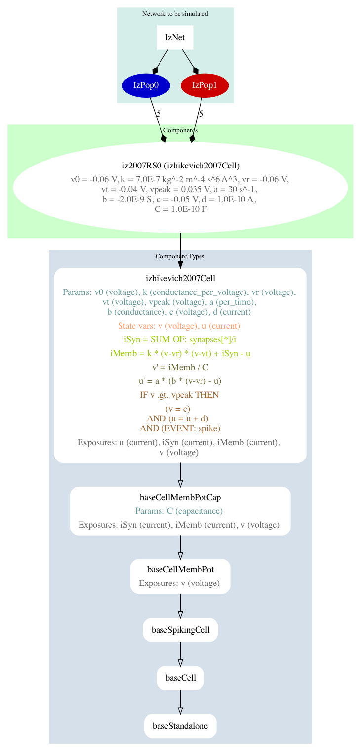
Fig. 12 A summary graph of the model generated using pynml -lems-graph.

It shows a top-down breakdown of the simulation: from the network, to the populations, to the cell types, leading up to the components that these cells are made of (more on Components later). Let us add the necessary code to run our simulation, this time using the well known NEURON simulator:

# Run the simulation
pynml.run_lems_with_jneuroml_neuron(
    lems_simulation_file, max_memory="2G", nogui=True, plot=False
)

Plotting recorded spike times

To analyse the outputs from the simulation, we can again plot the information we recorded. In the previous example, we had recorded and plotted the membrane potentials from our cell. Here, we have recorded the spike times. So let us plot them to generate our figure:

# Load the data from the file and plot the spike times
# using the pynml generate_plot utility function.
data_array_0 = np.loadtxt("%s.0.spikes.dat" % simulation_id)
data_array_1 = np.loadtxt("%s.1.spikes.dat" % simulation_id)
times_0 = data_array_0[:, 1]
times_1 = data_array_1[:, 1]
ids_0 = data_array_0[:, 0]
ids_1 = [id + size0 for id in data_array_1[:, 0]]
pynml.generate_plot(
    [times_0, times_1],
    [ids_0, ids_1],
    "Spike times",
    show_plot_already=False,
    save_figure_to="%s-spikes.png" % simulation_id,
    xaxis="time (s)",
    yaxis="cell ID",
    colors=["b", "r"],
    linewidths=["0", "0"],
    markers=[".", "."],
)

Observe how we are using the same generate_plot utility function as before: it is general enough to plot different recorded quantities. Under the hood, it passes this information to Python’s Matplotlib library. This produces the raster plot shown at the top of the page.

This concludes our second example. Here, we have seen how to create, simulate, and record from a simple two population network of single compartment point neurons. The next section is an interactive notebook that you can use to play with this example. After that we will move on to the next example: a neuron model using Hodgkin Huxley style ion channels.